第3节: 变换

Transforms

中文英文

在第2.1节中，我们讨论了坐标系统以及如何将坐标从一个坐标系统转换为另一个的可能性。在本节中，我们将更仔细地探讨这个想法，并且还将看看几何变换如何用于将图形对象放置到一个坐标系统中。

In Section 2.1, we discussed coordinate systems and how it is possible to transform coordinates from one coordinate system to another. In this section, we'll look at that idea a little more closely, and also look at how geometric transformations can be used to place graphics objects into a coordinate system.

2.3.1 视口和建模

Viewing and Modeling

中文英文

在典型的应用中，我们有一个由像素构成的矩形，其自然像素坐标用于显示图像。这个矩形称为视口(viewport)。我们还有一组几何对象，这些对象在可能不同的坐标系中定义，通常是使用实数坐标而不是整数。这些对象组成了我们想要查看的“场景”或“世界”，用于定义场景的坐标称为世界坐标(world coordinates)。

对于二维图形，世界位于一个平面上。不可能显示整个无限平面的图像。我们需要在平面上选择一些矩形区域来显示在图像中。让我们称这个矩形区域为窗口，或称为视窗(window)。坐标变换用于将窗口映射到视口中。

在这个图示中，T代表坐标变换。T是一个函数，它接受窗口中的世界坐标(x,y)并将它们映射到视口中的像素坐标T(x,y)。在这个例子中，你可以检查到：

T(x,y) = ( 800*(x+4)/8, 600*(3-y)/6 )

看一下窗口中角落坐标为(-1,2)和(3,-1)的矩形。当这个矩形在视口中显示时，它将显示为具有角落T(-1,2)和T(3,-1)的矩形。在这个例子中，T(-1,2) = (300,100) 以及 T(3,-1) = (700,400)。

我们以这种方式使用坐标变换是因为它允许我们选择一个对于描述我们想要显示的场景而言是自然的世界坐标系，而这比直接使用视口坐标更容易。沿着同样的思路，假设我们想要定义一些复杂的对象，并假设在我们的场景中会有几个该对象的副本。或者也许我们正在制作一个动画，并且希望该对象在不同帧中有不同的位置。我们希望选择一些方便的坐标系，并将其用于一劳永逸地定义对象。我们用于定义对象的坐标称为该对象的对象坐标(object coordinates)。当我们想要将对象放置到场景中时，我们需要将用于定义对象的对象坐标转换为我们用于场景的世界坐标系。我们需要的转换称为建模变换(modeling transformation)。这张图片说明了一个在其自己的对象坐标系中定义的对象，然后通过三种不同的建模变换映射到世界坐标系中：

记住，为了查看场景，还会有另一个转换，将对象从世界坐标中的视窗映射到视口中。

现在，请记住，视窗的选择决定了图像中显示场景的哪一部分。移动、调整大小，甚至旋转窗口都会给场景带来不同的视图。假设我们制作了几张同一辆汽车的图片：

这张图片上部的图像和左下角的图像之间发生了什么？实际上，有两种可能性：要么汽车向右移动，要么定义场景的视窗向左移动。这一点很重要，请确保你理解了它。（试试用你的手机相机。把它对准一些物体，向左走一步，注意一下相机取景器中的物体会发生什么变化：它们在照片中向右移动！）同样，在顶部图片和底部中间的图片之间会发生什么？要么汽车逆时针旋转，要么窗口顺时针旋转。（再次尝试使用相机——你可能想拍两张实际照片以便比较。）最后，从顶部图片到右下角的图片的变化可能是因为汽车变小了，也可能是因为窗口变大了。（在你的相机上，更大的窗口意味着你看到了更大的视野，你可以通过给相机加上变焦或者从你正在观看的物体后退来实现这一点。）

这里有一个重要的总体概念。当我们修改视窗时，我们改变了应用于视口的坐标系统。但实际上，这等同于保持该坐标系统不变，而是移动场景中的对象。不过，为了在最终图像中获得相同的效果，您必须对对象应用相反的变换（例如，向左移动窗口等同于将对象向右移动）。因此，在转换窗口和转换对象之间并没有本质区别。在数学上，您通过在某个自然坐标系统中给出坐标来指定几何基元，计算机会对这些坐标应用一系列变换，最终产生用于在图像中实际绘制基元的坐标。您会认为其中一些变换是建模变换，一些是坐标变换，但对于计算机来说，这都是一样的。

这里有一个实时演示，可以帮助您理解建模变换和视口变换之间的等价性。滑块控制应用于图片中对象的变换。在演示的底部部分，您可以看到一个较大的视图，其中上部图像的视口被表示为半透明的黑色矩形。阅读演示中的帮助文本以获取更多信息。

我们稍后会在书中多次回到这个概念，但无论如何，您可以看到几何变换是计算机图形学中的一个核心概念。让我们更详细地看看一些基本类型的变换。我们在二维图形中将使用的变换可以写成如下形式：

x1 = a*x + b*y + e
y1 = c*x + d*y + f

其中 (x,y) 表示变换应用前的某一点的坐标，(x1,y1) 是变换后的坐标。这个变换由六个常数 a、b、c、d、e 和 f 定义。注意，这可以写成一个函数 T，其中

T(x,y) = ( a*x + b*y + e, c*x + d*y + f )

这种形式的变换称为仿射变换。仿射变换具有以下性质：当它应用于两条平行线时，变换后的线也将是平行的。此外，如果将一个仿射变换跟随另一个仿射变换，结果仍然是一个仿射变换。

In a typical application, we have a rectangle made of pixels, with its natural pixel coordinates, where an image will be displayed. This rectangle will be called the viewport. We also have a set of geometric objects that are defined in a possibly different coordinate system, generally one that uses real-number coordinates rather than integers. These objects make up the "scene" or "world" that we want to view, and the coordinates that we use to define the scene are called world coordinates.

For 2D graphics, the world lies in a plane. It's not possible to show a picture of the entire infinite plane. We need to pick some rectangular area in the plane to display in the image. Let's call that rectangular area the window, or view window. A coordinate transform is used to map the window to the viewport.

In this illustration, T represents the coordinate transformation. T is a function that takes world coordinates (x,y) in some window and maps them to pixel coordinates T(x,y) in the viewport. (I've drawn the viewport and window with different sizes to emphasize that they are not the same thing, even though they show the same objects, but in fact they don't even exist in the same space, so it doesn't really make sense to compare their sizes.) In this example, as you can check,

T(x,y) = ( 800*(x+4)/8, 600*(3-y)/6 )

Look at the rectangle with corners at (-1,2) and (3,-1) in the window. When this rectangle is displayed in the viewport, it is displayed as the rectangle with corners T(-1,2) and T(3,-1). In this example, T(-1,2) = (300,100) and T(3,-1) = (700,400).

We use coordinate transformations in this way because it allows us to choose a world coordinate system that is natural for describing the scene that we want to display, and it is easier to do that than to work directly with viewport coordinates. Along the same lines, suppose that we want to define some complex object, and suppose that there will be several copies of that object in our scene. Or maybe we are making an animation, and we would like the object to have different positions in different frames. We would like to choose some convenient coordinate system and use it to define the object once and for all. The coordinates that we use to define an object are called object coordinates for the object. When we want to place the object into a scene, we need to transform the object coordinates that we used to define the object into the world coordinate system that we are using for the scene. The transformation that we need is called a modeling transformation. This picture illustrates an object defined in its own object coordinate system and then mapped by three different modeling transformations into the world coordinate system:

Remember that in order to view the scene, there will be another transformation that maps the object from a view window in world coordinates into the viewport.

Now, keep in mind that the choice of a view window tells which part of the scene is shown in the image. Moving, resizing, or even rotating the window will give a different view of the scene. Suppose we make several images of the same car:

What happened between making the top image in this illustration and making the image on the bottom left? In fact, there are two possibilities: Either the car was moved to the right, or the view window that defines the scene was moved to the left. This is important, so be sure you understand it. (Try it with your cell phone camera. Aim it at some objects, take a step to the left, and notice what happens to the objects in the camera's viewfinder: They move to the right in the picture!) Similarly, what happens between the top picture and the middle picture on the bottom? Either the car rotated counterclockwise, or the window was rotated clockwise. (Again, try it with a camera—you might want to take two actual photos so that you can compare them.) Finally, the change from the top picture to the one on the bottom right could happen because the car got smaller or because the window got larger. (On your camera, a bigger window means that you are seeing a larger field of view, and you can get that by applying a zoom to the camera or by backing up away from the objects that you are viewing.)

There is an important general idea here. When we modify the view window, we change the coordinate system that is applied to the viewport. But in fact, this is the same as leaving that coordinate system in place and moving the objects in the scene instead. Except that to get the same effect in the final image, you have to apply the opposite transformation to the objects (for example, moving the window to the left is equivalent to moving the objects to the right). So, there is no essential distinction between transforming the window and transforming the object. Mathematically, you specify a geometric primitive by giving coordinates in some natural coordinate system, and the computer applies a sequence of transformations to those coordinates to produce, in the end, the coordinates that are used to actually draw the primitive in the image. You will think of some of those transformations as modeling transforms and some as coordinate transforms, but to the computer, it's all the same.

Here is a live demo that can help you to understand the equivalence between modeling transformations and viewport transformations. The sliders control transformations that are applied to the objects in the picture. In the lower section of the demo, you see a larger view in which the viewport for the upper image is represented as a translucent black rectangle. Read the help text in the demo for more information.

We will return to this idea several times later in the book, but in any case, you can see that geometric transforms are a central concept in computer graphics. Let's look at some basic types of transformation in more detail. The transforms we will use in 2D graphics can be written in the form

x1 = a*x + b*y + e
y1 = c*x + d*y + f

where (x,y) represents the coordinates of some point before the transformation is applied, and (x1,y1) are the transformed coordinates. The transform is defined by the six constants a, b, c, d, e, and f. Note that this can be written as a function T, where

T(x,y) = ( a*x + b*y + e, c*x + d*y + f )

A transformation of this form is called an affine transform. An affine transform has the property that, when it is applied to two parallel lines, the transformed lines will also be parallel. Also, if you follow one affine transform by another affine transform, the result is again an affine transform.

2.3.2 平移

Translation

中文英文

平移变换简单地将每个点水平移动一定量，垂直移动一定量。如果 (x,y) 是原始点，(x1,y1) 是变换后的点，那么平移的公式为

x1 = x + e
y1 = y + f

其中 e 是点水平移动的单位数，f 是垂直移动的单位数。（因此，对于平移，仿射变换的一般公式中 a = d = 1，b = c = 0。）一个二维图形系统通常会有一个类似于

translate( e, f )

的函数来应用平移变换。平移将应用于在给出命令后绘制的所有内容。也就是说，对于所有后续的绘图操作，e 将被添加到 x 坐标，f 将被添加到 y 坐标。让我们看一个例子。假设你使用以 (0,0) 为中心的坐标绘制一个“F”。如果在绘制“F”之前说 translate(4,2)，那么在实际使用坐标之前，“F”的每个点都将水平移动 4 个单位，垂直移动 2 个单位，因此在平移之后，“F”将位于 (4,2)：

这张图片中浅灰色的“F”显示了在没有平移的情况下会绘制什么；深红色的“F”显示了应用了平移 (4,2) 后绘制的相同的“F”。顶部的箭头显示了“F”的左上角已向右移动 4 个单位，向上移动 2 个单位。在“F”中的每个点都受到相同的位移影响。请注意，在我的例子中，我假设 y 坐标从下到上递增。也就是说，y 轴朝上。

记住，当你给出 translate(e,f) 命令时，这个平移将应用于之后所有的绘图，而不仅仅是下一个你绘制的形状。如果你在平移后应用另一个变换，第二个变换不会取代平移，而是与平移结合起来，从而后续的绘图将受到组合变换的影响。例如，如果你将 translate(4,2) 与 translate(-1,5) 组合，结果与单个平移 translate(3,7) 相同。这是一个重要的观点，稍后将会有更多内容介绍。

还要记住，你不需要自己计算坐标变换。你只需要为对象指定原始坐标（即对象坐标），并指定要应用的变换或变换。计算机会负责将变换应用于坐标。你甚至不需要知道用于变换的方程式；你只需要理解它在几何上做了什么。

A translation transform simply moves every point by a certain amount horizontally and a certain amount vertically. If (x,y) is the original point and (x1,y1) is the transformed point, then the formula for a translation is

x1 = x + e
y1 = y + f
‵‵‵

where e is the number of units by which the point is moved horizontally and f is the amount by which it is moved vertically. (Thus for a translation, a = d = 1, and b = c = 0 in the general formula for an affine transform.) A 2D graphics system will typically have a function such as

```text
translate( e, f )

to apply a translate transformation. The translation would apply to everything that is drawn after the command is given. That is, for all subsequent drawing operations, e would be added to the x-coordinate and f would be added to the y-coordinate. Let's look at an example. Suppose that you draw an "F" using coordinates in which the "F" is centered at (0,0). If you say translate(4,2) before drawing the "F", then every point of the "F" will be moved horizontally by 4 units and vertically by 2 units before the coordinates are actually used, so that after the translation, the "F" will be centered at (4,2):

The light gray "F" in this picture shows what would be drawn without the translation; the dark red "F" shows the same "F" drawn after applying a translation by (4,2). The top arrow shows that the upper left corner of the "F" has been moved over 4 units and up 2 units. Every point in the "F" is subjected to the same displacement. Note that in my examples, I am assuming that the y-coordinate increases from bottom to top. That is, the y-axis points up.

Remember that when you give the command translate(e,f), the translation applies to all the drawing that you do after that, not just to the next shape that you draw. If you apply another transformation after the translation, the second transform will not replace the translation. It will be combined with the translation, so that subsequent drawing will be affected by the combined transformation. For example, if you combine translate(4,2) with translate(-1,5), the result is the same as a single translation, translate(3,7). This is an important point, and there will be a lot more to say about it later.

Also remember that you don't compute coordinate transformations yourself. You just specify the original coordinates for the object (that is, the object coordinates), and you specify the transform or transforms that are to be applied. The computer takes care of applying the transformation to the coordinates. You don't even need to know the equations that are used for the transformation; you just need to understand what it does geometrically.

2.3.3 旋转

Rotation

中文英文

在我们这里的情况下，旋转变换会围绕原点 (0,0) 旋转每个点。每个点都被旋转相同的角度，称为旋转角度。为此，角度可以用度或弧度来度量。（我们稍后将在本章中查看的 Java 和 JavaScript 的 2D 图形 API 使用弧度，但 OpenGL 和 SVG 使用度。）具有正角度的旋转会将对象顺时针旋转从正 x 轴指向正 y 轴的方向。在这里的示例中，坐标系中 y 轴向上，这是逆时针旋转，但在通常的像素坐标中，y 轴向下而不是向上，所以这是顺时针旋转。虽然不明显，但是当对点 (x,y) 应用以 r 弧度为角度的绕原点旋转时，结果点 (x1,y1) 由以下公式给出：

x1 = cos(r) * x - sin(r) * y
y1 = sin(r) * x + cos(r) * y

也就是说，在仿射变换的一般公式中，e = f = 0，a = d = cos(r)，b = -sin(r)，c = sin(r)。这里有一个图示，说明了绕原点旋转负 135 度的角度：

再次，浅灰色的“F”是原始形状，深红色的“F”是应用旋转后的形状。箭头显示了原始“F”的左上角是如何移动的。

一个 2D 图形 API 通常会有一个 rotate(r) 命令来应用旋转。这个命令在绘制应用旋转的对象之前使用。

A rotation transform, for our purposes here, rotates each point about the origin, (0,0). Every point is rotated through the same angle, called the angle of rotation. For this purpose, angles can be measured either in degrees or in radians. (The 2D graphics APIs for Java and JavaScript that we will look at later in this chapter use radians, but OpenGL and SVG use degrees.) A rotation with a positive angle rotates objects in the direction from the positive x-axis towards the positive y-axis. This is counterclockwise in a coordinate system where the y-axis points up, as it does in my examples here, but it is clockwise in the usual pixel coordinates, where the y-axis points down rather than up. Although it is not obvious, when rotation through an angle of r radians about the origin is applied to the point (x,y), then the resulting point (x1,y1) is given by

```text x1 = cos(r) * x - sin(r) * y y1 = sin(r) * x + cos(r) * y ‵‵‵

That is, in the general formula for an affine transform, e = f = 0, a = d = cos(r), b = -sin(r), and c = sin(r). Here is a picture that illustrates a rotation about the origin by the angle negative 135 degrees:

Again, the light gray "F" is the original shape, and the dark red "F" is the shape that results if you apply the rotation. The arrow shows how the upper left corner of the original "F" has been moved.

A 2D graphics API would typically have a command rotate(r) to apply a rotation. The command is used before drawing the objects to which the rotation applies.

2.3.4 组合变换

Combining Transformations

中文英文

现在我们可以看到当你组合两个变换时会发生什么。假设在绘制某个对象之前，你说：

translate(4,0)
rotate(90)

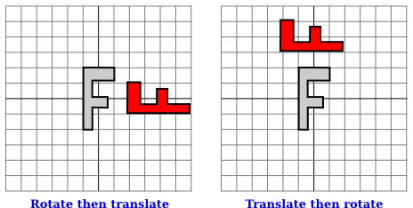
假设角度是以度为单位测量的。然后平移将应用于所有后续的绘制。但是，由于旋转命令，你在平移之后绘制的东西是旋转的对象。也就是说，平移应用于已经旋转过的对象。下图的左侧是一个例子，在这个例子中，浅灰色的“F”是原始形状，红色的“F”显示了将这两个变换应用于原始形状的结果。原始“F”首先被旋转了90度角度，然后向右移动了4个单位。

请注意，变换是以与代码中给出的顺序相反的顺序应用于对象的（因为代码中的第一个变换是应用于已经受到第二个变换影响的对象）。还请注意，应用变换的顺序很重要。如果我们在这个例子中颠倒两个变换的应用顺序，通过以下方式：

rotate(90)
translate(4,0)

那么结果就如上图右侧所示。在那张图片中，原始“F”首先向右移动4个单位，然后通过原点旋转90度角度，以得到实际显示在屏幕上的形状。

对于另一个应用多个变换的例子，假设我们想要围绕点 (p,q) 而不是围绕点 (0,0) 将一个形状旋转 r 角度。我们可以通过首先将点 (p,q) 移动到原点，使用 translate(-p,-q) 来实现这一点。然后我们可以调用 rotate(r) 进行围绕原点的标准旋转。最后，我们可以通过应用 translate(p,q) 将原点移回点 (p,q)。记住我们必须以相反的顺序编写变换的代码，我们需要在绘制形状之前说：

translate(p,q)
rotate(r)
translate(-p,-q)

（事实上，一些图形 API 允许我们使用单个命令来实现这个变换，例如 rotate(r,p,q)。这将在点 (p,q) 处围绕角度 r 进行旋转。）

We are now in a position to see what can happen when you combine two transformations. Suppose that before drawing some object, you say

translate(4,0)
rotate(90)
‵‵‵

Assume that angles are measured in degrees. The translation will then apply to all subsequent drawing. But, because of the rotation command, the things that you draw after the translation are rotated objects. That is, the translation applies to objects that have already been rotated. An example is shown on the left in the illustration below, where the light gray "F" is the original shape, and red "F" shows the result of applying the two transforms to the original. The original "F" was first rotated through a 90 degree angle, and then moved 4 units to the right.

<figure markdown="span">
    ![pixel-coordinates](../../en/c2/rotate-and-translate-2d.png)
</figure>

Note that transforms are applied to objects in the reverse of the order in which they are given in the code (because the first transform in the code is applied to an object that has already been affected by the second transform). And note that the order in which the transforms are applied is important. If we reverse the order in which the two transforms are applied in this example, by saying

```text
rotate(90)
translate(4,0)
‵‵‵

then the result is as shown on the right in the above illustration. In that picture, the original "F" is first moved 4 units to the right and the resulting shape is then rotated through an angle of 90 degrees about the origin to give the shape that actually appears on the screen.

For another example of applying several transformations, suppose that we want to rotate a shape through an angle r about a point (p,q) instead of about the point (0,0). We can do this by first moving the point (p,q) to the origin, using translate(-p,-q). Then we can do a standard rotation about the origin by calling rotate(r). Finally, we can move the origin back to the point (p,q) by applying translate(p,q). Keeping in mind that we have to write the code for the transformations in the reverse order, we need to say

```text
translate(p,q)
rotate(r)
translate(-p,-q)

before drawing the shape. (In fact, some graphics APIs let us accomplish this transform with a single command such as rotate(r,p,q). This would apply a rotation through the angle r about the point (p,q).)

2.3.5 缩放

Scaling

中文英文

缩放变换可用于使对象变大或变小。在数学上，缩放变换简单地将每个 x 坐标乘以一个给定的量，每个 y 坐标乘以一个给定的量。也就是说，如果一个点 (x,y) 在 x 方向上按比例因子 a 缩放，在 y 方向上按比例因子 d 缩放，那么结果点 (x1,y1) 由以下公式给出：

x1 = a * x
y1 = d * y

如果将此变换应用于以原点为中心的形状，则会将形状在水平方向上拉伸 a 倍，垂直方向上拉伸 d 倍。以下是一个示例，原始的浅灰色“F”在水平方向上按 3 倍，垂直方向上按 2 倍进行缩放，得到最终的深红色“F”：

常见情况是水平和垂直缩放因子相同，称为均匀缩放(uniform scaling)。均匀缩放拉伸或收缩一个形状而不会扭曲它。

当缩放应用于不以 (0,0) 为中心的形状时，除了被拉伸或收缩之外，形状还将远离或接近 0。事实上，缩放操作的真实描述是将每个点远离 (0,0) 或将每个点拉向 (0,0)。如果想要围绕不同于 (0,0) 的点进行缩放，可以使用与旋转情况类似的三个变换的序列。

一个 2D 图形 API 可以提供一个名为 scale(a,d) 的函数来应用缩放变换。与往常一样，该变换应用于所有后续绘图操作中的所有 x 和 y 坐标。请注意，允许使用负缩放因子，并且会导致反射形状以及可能的拉伸或收缩。例如，scale(1,-1) 将使对象在垂直方向上反射，通过 x 轴。

事实上，每个仿射变换都可以通过组合平移、绕原点旋转和原点缩放来创建。我不会试图证明这一点，但下面是一个交互式演示，让您可以尝试平移、旋转和缩放，并尝试组合它们所产生的变换。

我还注意到，由平移和绕原点旋转构成的变换，没有缩放，将保持被应用对象的长度和角度。它也会保持矩形的纵横比。具有这种属性的变换被称为“欧几里得”。如果还允许均匀缩放，则结果变换将保持角度和纵横比，但不会保持长度。

A scaling transform can be used to make objects bigger or smaller. Mathematically, a scaling transform simply multiplies each x-coordinate by a given amount and each y-coordinate by a given amount. That is, if a point (x,y) is scaled by a factor of a in the x direction and by a factor of d in the y direction, then the resulting point (x1,y1) is given by

x1 = a * x
y1 = d * y

If you apply this transform to a shape that is centered at the origin, it will stretch the shape by a factor of a horizontally and d vertically. Here is an example, in which the original light gray "F" is scaled by a factor of 3 horizontally and 2 vertically to give the final dark red "F":

The common case where the horizontal and vertical scaling factors are the same is called uniform scaling. Uniform scaling stretches or shrinks a shape without distorting it.

When scaling is applied to a shape that is not centered at (0,0), then in addition to being stretched or shrunk, the shape will be moved away from 0 or towards 0. In fact, the true description of a scaling operation is that it pushes every point away from (0,0) or pulls every point towards (0,0). If you want to scale about a point other than (0,0), you can use a sequence of three transforms, similar to what was done in the case of rotation.

A 2D graphics API can provide a function scale(a,d) for applying scaling transformations. As usual, the transform applies to all x and y coordinates in subsequent drawing operations. Note that negative scaling factors are allowed and will result in reflecting the shape as well as possibly stretching or shrinking it. For example, scale(1,-1) will reflect objects vertically, through the x-axis.

It is a fact that every affine transform can be created by combining translations, rotations about the origin, and scalings about the origin. I won't try to prove that, but here is an interactive demo that will let you experiment with translations, rotations, and scalings, and with the transformations that can be made by combining them.

I also note that a transform that is made from translations and rotations, with no scaling, will preserve length and angles in the objects to which it is applied. It will also preserve aspect ratios of rectangles. Transforms with this property are called "Euclidean." If you also allow uniform scaling, the resulting transformation will preserve angles and aspect ratio, but not lengths.

2.3.6 剪切

Shear

中文英文

我们将再看一个基本变换类型，剪切变换。尽管必要时可以通过旋转和缩放来构建剪切，但如何做到这一点并不是很明显。剪切会“倾斜”对象。水平剪切会将事物向左（负剪切）或向右（正剪切）倾斜。垂直剪切会使它们向上或向下倾斜。以下是水平剪切的示例：

水平剪切不会移动 x 轴。每条水平线都会根据该线上的 y 值移动到左侧或右侧。当将水平剪切应用于点 (x,y) 时，得到的结果点 (x1,y1) 由以下公式给出：

x1 = x + b * y
y1 = y

其中 b 是某个常数剪切因子。类似地，具有剪切因子 c 的垂直剪切由以下方程给出：

x1 = x
y1 = c * x + y

剪切有时被称为“倾斜”，但倾斜通常是指一个角度，而不是一个剪切因子。

We will look at one more type of basic transform, a shearing transform. Although shears can in fact be built up out of rotations and scalings if necessary, it is not really obvious how to do so. A shear will "tilt" objects. A horizontal shear will tilt things towards the left (for negative shear) or right (for positive shear). A vertical shear tilts them up or down. Here is an example of horizontal shear:

A horizontal shear does not move the x-axis. Every other horizontal line is moved to the left or to the right by an amount that is proportional to the y-value along that line. When a horizontal shear is applied to a point (x,y), the resulting point (x1,y1) is given by

x1 = x + b * y
y1 = y

for some constant shearing factor b. Similarly, a vertical shear with shearing factor c is given by the equations

x1 = x
y1 = c * x + y

Shear is occasionally called "skew," but skew is usually specified as an angle rather than as a shear factor.

2.3.7 视窗到视口

Window-to-Viewport

中文英文

在图像显示之前应用于对象的最后一个变换是窗口到视口变换，它将包含场景的 xy 平面中的矩形视窗映射到图像将显示的像素矩形网格中。我在这里假设视窗没有旋转；也就是说，它的边是平行于 x 和 y 轴的。在这种情况下，窗口到视口变换可以用平移和缩放变换来表示。让我们看看典型情况，其中视口具有从左边的 0 到右边的宽度、从顶部的 0 到底部的高度的像素坐标。并假设视窗的限制是 left、right、bottom 和 top。在这种情况下，窗口到视口变换可以编程为：

scale( width / (right-left), height / (bottom-top) );
translate( -left, -top )

这些应该是应用于点的最后变换。由于变换是按与程序中指定的顺序相反的顺序应用于点的，它们应该是程序中指定的第一个变换。为了看到这是如何工作的，请考虑视窗中的一个点 (x,y)。（这个点来自场景中的某个对象。可能已经应用了几次建模变换来生成点 (x,y)，而该点现在已准备好进行最终的转换为视口坐标。）坐标 (x,y) 首先被平移了 (-left,-top) 以得到 (x-left,y-top)。然后将这些坐标乘以上面显示的缩放因子，得到最终的坐标：

x1 = width / (right-left) * (x-left)
y1 = height / (bottom-top) * (y-top)

请注意，点 (left,top) 被映射到 (0,0)，而点 (right,bottom) 被映射到 (width,height)，这正是我们想要的。

还有一个纵横比的问题。如 2.1.3 小节 所述，如果我们希望强制窗口的纵横比与视口的纵横比匹配，可能需要调整窗口的限制。下面是一个子程序的伪代码，假设视口的左上角具有像素坐标 (0,0)：

subroutine applyWindowToViewportTransformation (
        left, right,   // horizontal limits on view window
        bottom, top,   // vertical limits on view window
        width, height, // width and height of viewport
        preserveAspect // should window be forced to match viewport aspect?
    )

if preserveAspect :
    // Adjust the limits to match the aspect ratio of the drawing area.
    displayAspect = abs(height / width);
    windowAspect = abs(( top-bottom ) / ( right-left ));
    if displayAspect > windowAspect :
        // Expand the viewport vertically.
        excess = (top-bottom) * (displayAspect/windowAspect - 1)
        top = top + excess/2
        bottom = bottom - excess/2
    else if displayAspect < windowAspect :
        // Expand the viewport horizontally.
        excess = (right-left) * (windowAspect/displayAspect - 1)
        right = right + excess/2
        left = left - excess/2 

    scale( width / (right-left), height / (bottom-top) )
    translate( -left, -top )

The last transformation that is applied to an object before it is displayed in an image is the window-to-viewport transformation, which maps the rectangular view window in the xy-plane that contains the scene to the rectangular grid of pixels where the image will be displayed. I'll assume here that the view window is not rotated; that it, its sides are parallel to the x- and y-axes. In that case, the window-to-viewport transformation can be expressed in terms of translation and scaling transforms. Let's look at the typical case where the viewport has pixel coordinates ranging from 0 on the left to width on the right and from 0 at the top to height at the bottom. And assume that the limits on the view window are left, right, bottom, and top. In that case, the window-to-viewport transformation can be programmed as:

scale( width / (right-left), height / (bottom-top) );
translate( -left, -top )

These should be the last transforms that are applied to a point. Since transforms are applied to points in the reverse of the order in which they are specified in the program, they should be the first transforms that are specified in the program. To see how this works, consider a point (x,y) in the view window. (This point comes from some object in the scene. Several modeling transforms might have already been applied to the object to produce the point (x,y), and that point is now ready for its final transformation into viewport coordinates.) The coordinates (x,y) are first translated by (-left,-top) to give (x-left,y-top). These coordinates are then multiplied by the scaling factors shown above, giving the final coordinates

x1 = width / (right-left) * (x-left)
y1 = height / (bottom-top) * (y-top)

Note that the point (left,top) is mapped to (0,0), while the point (right,bottom) is mapped to (width,height), which is just what we want.

There is still the question of aspect ratio. As noted in Subsection 2.1.3, if we want to force the aspect ratio of the window to match the aspect ratio of the viewport, it might be necessary to adjust the limits on the window. Here is pseudocode for a subroutine that will do that, again assuming that the top-left corner of the viewport has pixel coordinates (0,0):

subroutine applyWindowToViewportTransformation (
        left, right,   // horizontal limits on view window
        bottom, top,   // vertical limits on view window
        width, height, // width and height of viewport
        preserveAspect // should window be forced to match viewport aspect?
    )

if preserveAspect :
    // Adjust the limits to match the aspect ratio of the drawing area.
    displayAspect = abs(height / width);
    windowAspect = abs(( top-bottom ) / ( right-left ));
    if displayAspect > windowAspect :
        // Expand the viewport vertically.
        excess = (top-bottom) * (displayAspect/windowAspect - 1)
        top = top + excess/2
        bottom = bottom - excess/2
    else if displayAspect < windowAspect :
        // Expand the viewport horizontally.
        excess = (right-left) * (windowAspect/displayAspect - 1)
        right = right + excess/2
        left = left - excess/2 

    scale( width / (right-left), height / (bottom-top) )
    translate( -left, -top )

2.3.8 矩阵和向量

Matrices and Vectors

中文英文

在计算机图形中使用的变换可以表示为矩阵，而它们作用的点则表示为向量。回想一下，从计算机科学家的角度来看，矩阵(matrix)是一个二维数组，而向量(vector)是一个一维数组。矩阵和向量是线性代数(linear algebra)领域的研究对象。线性代数对计算机图形至关重要。事实上，矩阵和向量数学已经内置在了 GPU 中。你不需要对线性代数有很多了解来阅读本教材，但一些基本概念是必不可少的。

我们需要的向量是由两个、三个或四个数字组成的列表。它们通常被写作 (x,y)、(x,y,z) 和 (x,y,z,w)。一个具有 N 行和 M 列的矩阵称为“N行M列矩阵”。在大多数情况下，我们需要的矩阵是 N 行 N 列的矩阵，其中 N 为 2、3 或 4。也就是说，它们有 2、3 或 4 行和列，行数等于列数。

如果 A 和 B 是两个 N 行 N 列的矩阵，那么它们可以相乘得到一个乘积矩阵 C = AB。如果 A 是一个 N 行 N 列的矩阵，v 是长度为 N 的向量，那么 v 可以乘以 A 得到另一个向量 w = Av。将 v 映射到 Av 的函数是一个变换；它将任意给定的大小为 N 的向量转换为另一个大小为 N 的向量。这种形式的变换称为线性变换(linear transformation)。

现在，假设 A 和 B 是 N 行 N 列的矩阵，v 是长度为 N 的向量。那么，我们可以形成两个不同的乘积：A(Bv) 和 (AB)v。一个核心事实是，这两个操作具有相同的效果。也就是说，我们可以先将 v 乘以 B，然后将结果乘以 A，或者我们可以将矩阵 A 和 B 相乘得到矩阵乘积 AB，然后将 v 乘以 AB。结果是相同的。

事实证明，旋转和缩放都是线性变换。也就是说，绕原点旋转 (x,y) 角度为 d 的操作可以通过将 (x,y) 乘以一个 2×2 的矩阵来实现。让我们称该矩阵为 Rd。类似地，水平方向缩放因子为 a，垂直方向缩放因子为 b，可以表示为一个矩阵 Sa,b。如果我们想对点 v = (x,y) 应用缩放后再旋转，我们可以计算要么 Rd(Sa,b^v) 要么 (RdSa,b)v。

那么呢？嗯，假设我们想要对数千个点应用相同的两个操作，先缩放再旋转，就像我们在为计算机图形中的对象进行变换时通常所做的那样。关键在于，我们可以一劳永逸地计算乘积矩阵 RdSa,b，然后通过单次乘法将组合变换应用于每个点。这意味着如果一个程序说

rotate(d)
scale(a,b)
.
.  // draw a complex object
.

计算机无需跟踪两个独立的操作。它将这些操作合并成一个单独的矩阵，然后只需跟踪这个矩阵。即使对对象应用了50个变换，计算机也可以将它们全部合并成一个矩阵。通过使用矩阵代数，多个变换可以像单个变换一样高效地处理！

这确实很好，但存在一个严重的问题：平移不是线性变换。为了将平移纳入这个框架，我们首先做一些看起来有点奇怪的事情：我们不再将二维点表示为一对数字 (x,y)，而是表示为三个数字的三元组 (x,y,1)。也就是说，我们在第三个坐标位置添加了一个 1。然后，结果是我们可以将旋转、缩放和平移——因此任何仿射变换——在二维空间中表示为一个 3×3 矩阵的乘法。我们需要的矩阵具有包含 (0,0,1) 的底部一行。将 (x,y,1) 乘以这样的矩阵会得到一个新向量 (x1,y1,1)。我们忽略额外的坐标，并将其视为将 (x,y) 转换为 (x1,y1)。有关记录，2D 平移 (Ta,b)、缩放 (Sa,b) 和旋转 (Rd) 的 3×3 矩阵如下所示：

你可以将这些矩阵的乘法与上面给出的平移、缩放和旋转公式进行比较。但在进行图形编程时，你不需要自己执行这些乘法。目前，你应该从这次讨论中带走的重要观点是，一系列变换可以合并成单个变换。计算机只需要跟踪一个矩阵，我们可以称之为“当前矩阵”或“当前变换”。为了实现诸如 translate(a,b) 或 rotate(d) 等变换命令，计算机只需将当前矩阵乘以代表变换的矩阵。

The transforms that are used in computer graphics can be represented as matrices, and the points on which they operate are represented as vectors. Recall that a matrix, from the point of view of a computer scientist, is a two-dimensional array of numbers, while a vector is a one-dimensional array. Matrices and vectors are studied in the field of mathematics called linear algebra. Linear algebra is fundamental to computer graphics. In fact, matrix and vector math is built into GPUs. You won't need to know a great deal about linear algebra for this textbook, but a few basic ideas are essential.

The vectors that we need are lists of two, three, or four numbers. They are often written as (x,y), (x,y,z), and (x,y,z,w). A matrix with N rows and M columns is called an "N-by-M matrix." For the most part, the matrices that we need are N-by-N matrices, where N is 2, 3, or 4. That is, they have 2, 3, or 4 rows and columns, and the number of rows is equal to the number of columns.

If A and B are two N-by-N matrices, then they can be multiplied to give a product matrix C = AB. If A is an N-by-N matrix, and v is a vector of length N, then v can be multiplied by A to give another vector w = Av. The function that takes v to Av is a transformation; it transforms any given vector of size N into another vector of size N. A transformation of this form is called a linear transformation.

Now, suppose that A and B are N-by-N matrices and v is a vector of length N. Then, we can form two different products: A(Bv) and (AB)v. It is a central fact that these two operations have the same effect. That is, we can multiply v by B and then multiply the result by A, or we can multiply the matrices A and B to get the matrix product AB and then multiply v by AB. The result is the same.

Rotation and scaling, as it turns out, are linear transformations. That is, the operation of rotating (x,y) through an angle d about the origin can be done by multiplying (x,y) by a 2-by-2 matrix. Let's call that matrix Rd. Similarly, scaling by a factor a in the horizontal direction and b in the vertical direction can be given as a matrix Sa,b. If we want to apply a scaling followed by a rotation to the point v = (x,y), we can compute either Rd(Sa,b^v) or (RdSa,b)v.

So what? Well, suppose that we want to apply the same two operations, scale then rotate, to thousands of points, as we typically do when transforming objects for computer graphics. The point is that we could compute the product matrix RdSa,b once and for all, and then apply the combined transform to each point with a single multiplication. This means that if a program says

rotate(d)
scale(a,b)
.
.  // draw a complex object
.

the computer doesn't have to keep track of two separate operations. It combines the operations into a single matrix and just keeps track of that. Even if you apply, say, 50 transformations to the object, the computer can just combine them all into one matrix. By using matrix algebra, multiple transformations can be handled as efficiently as a single transformation!

This is really nice, but there is a gaping problem: Translation is not a linear transformation. To bring translation into this framework, we do something that looks a little strange at first: Instead of representing a point in 2D as a pair of numbers (x,y), we represent it as the triple of numbers (x,y,1). That is, we add a one as the third coordinate. It then turns out that we can then represent rotation, scaling, and translation—and hence any affine transformation—on 2D space as multiplication by a 3-by-3 matrix. The matrices that we need have a bottom row containing (0,0,1). Multiplying (x,y,1) by such a matrix gives a new vector (x1,y1,1). We ignore the extra coordinate and consider this to be a transformation of (x,y) into (x1,y1). For the record, the 3-by-3 matrices for translation (Ta,b), scaling (Sa,b), and rotation (Rd) in 2D are

You can compare multiplication by these matrices to the formulas given above for translation, scaling, and rotation. But when doing graphics programming, you won't need to do the multiplication yourself. For now, the important idea that you should take away from this discussion is that a sequence of transformations can be combined into a single transformation. The computer only needs to keep track of a single matrix, which we can call the "current matrix" or "current transformation." To implement transform commands such as translate(a,b) or rotate(d), the computer simply multiplies the current matrix by the matrix that represents the transform.