附录 B#
Appendix B
使用 Gnuplot 绘图#
Graphing with Gnuplot
Gnuplot 是一个免费的开源软件包,用于生成各种图形。它有适用于多种操作系统的版本。下面是一个简要教程,介绍如何使用 Gnuplot 绘制三角函数图像。
Gnuplot is a free, open-source software package for producing a variety of graphs. Versions are available for many operating systems. Below is a very brief tutorial on how to use Gnuplot to graph trigonometric functions.
安装#
INSTALLATION
访问 http://www.gnuplot.info/download.html,按照链接下载适用于你的操作系统的最新版本。对于 Windows,你应下载名为类似
gp460-win32-setup.exe的安装文件(即版本 4.6.0)。这里讨论的所有示例都假设至少是 4.6.0 版本,尽管它们在早期的 4.x 版本中通常也能运行。安装下载的文件。例如,在 Windows 中运行你在第 1 步下载的安装文件,默认将 Gnuplot 安装在
C:\symbol{92}Program Files\gnuplot文件夹中。你可以接受默认设置,但应在 选择附加任务 界面中选择 “创建桌面图标” 选项。(可选)阅读 http://gnuplot.info/documentation.html 上的文档。
Go to http://www.gnuplot.info/download.html and follow the links to download the latest version for your operating system. For Windows, you should download the setup file with a name such as
gp460-win32-setup.exe, which is version 4.6.0. All the examples discussed here will assume at least version 4.6.0, though they should work with earlier 4.x versions.Install the downloaded file. For example, in Windows you would run the setup file you downloaded in Step 1, which installs Gnuplot in the
C:\symbol{92}Program Files\gnuplotfolder by default. You can accept the defaults during installation, though you should select the “Create a desktop icon” option in the Select Additional Tasks screen.(Optional) Read the documentation at http://gnuplot.info/documentation.html.
运行 Gnuplot#
RUNNING GNUPLOT
在 Windows 中,从你安装 Gnuplot 的
bin文件夹中运行wgnuplot.exe``(默认位置是 ``C:\Program Files\gnuplot\bin\wgnuplot.exe),或者如果你在安装时选择了该选项,也可以双击桌面图标。在 Linux 中,只需在终端窗口中输入gnuplot。你现在应该能看到一个带有
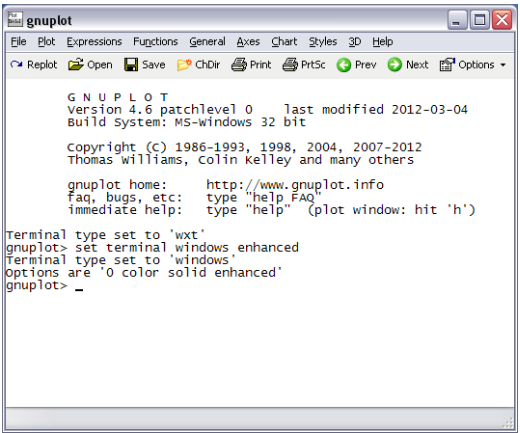
gnuplot>命令提示符的 Gnuplot 终端。在 Windows 中,它会出现在一个新窗口中,如下一页所示的图片。在 Linux 中,它会出现在运行gnuplot命令的终端窗口中。对于 Windows,如果字体难以辨认,可以通过右键点击 Gnuplot 窗口的文本区域并选择 “选择字体…” 选项进行更改。例如,字体选择 “Courier”,样式 “Regular”,字号 “12” 通常是一个不错的选择(可以通过再次右键点击 Gnuplot 窗口并选择更新 wgnuplot.ini 的选项来保存该设置,以便下次会话使用)。现在在
gnuplot>命令提示符下,你可以运行绘图命令,下面将对其进行说明。
函数绘图
在 Gnuplot 中创建图像的常用方式是使用 plot 命令:
对于一个函数 \(y=f(x)\),<range> 是用于绘图的 \(x\) 值范围(可选地也包括 \(y\) 值范围)。若要指定一个 \(x\) 范围,使用形式为 \([a:b]\) 的表达式,其中 \(a<b\)。这将使图像在 \(a\le x\le b\) 的区间内绘制。
若要同时指定 \(x\) 范围和 \(y\) 范围,使用形式为 \([a:b]\) \([c:d]\) 的表达式,其中 \(a<b\) 且 \(c<d\)。这将使图像在 \(a\le x\le b\) 且 \(c\le y \le d\) 的区间内绘制。
函数定义使用 \(x\) 变量与下列数学运算符组合:
符号 |
操作 |
示例 |
结果 |
\(+\) |
加法 |
\(2 + 3\) |
\(5\) |
\(-\) |
减法 |
\(3 - 2\) |
\(1\) |
* |
乘法 |
\(2`*`3\) |
\(6\) |
\(/\) |
除法 |
\(4/2\) |
\(2\) |
** |
平方 |
\(2\) ** \(3\) |
\(2^3 = 8\) |
exp(\(x\)) |
\(e^x\) |
exp(\(2\)) |
\(e^2\) |
log(\(x\)) |
\(\ln x\) |
log(\(2\)) |
\(\ln 2\) |
sin(\(x\)) |
\(\sin x\) |
sin(pi/\(2\)) |
\(1\) |
cos(\(x\)) |
\(\cos x\) |
cos(pi) |
\(-1\) |
tan(\(x\)) |
\(\tan x\) |
tan(pi/\(4\)) |
\(1\) |
注意我们使用特殊关键字 “pi” 来表示 \(\pi\) 的值。
示例 B.1.
要绘制函数 \(y=\sin\;x\) 在区间 \(x=0\) 到 \(x=2\pi\) 上的图像,在 gnuplot 提示符下输入:
结果如下图所示:
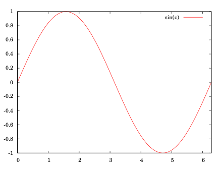
注意 \(x\) 轴标注为整数。若要将 \(x\) 轴标注为 \(\pi\) 的分数形式,需要修改 terminal 设置。在 Windows 中,可以使用如下命令:
在 Linux 中则使用:
然后(前提是系统已安装 Symbol 字体,通常已安装)可使用以下命令(需一行输入)将 \(x\) 轴标注为从 \(0\) 到 \(2\pi\) 的 \(\pi/2\) 的倍数:
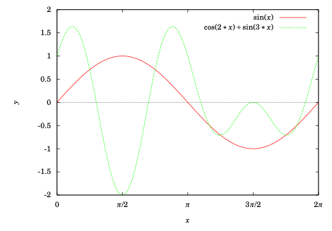
在上面的示例中,若要在同一图像中绘制函数 \(y=\cos\;2x + \sin\;3x\),可在第一个函数后加一个逗号并添加新函数:
默认情况下,图像中不会显示 x 轴。若要显示它,请在 plot 命令 之前 输入以下命令:
此外,若要为坐标轴添加标签,请使用如下命令:
绘图默认的采样数量为 \(100\),对于复杂曲线可能会导致边缘不平滑。为了获得更平滑的曲线,可将采样数增加(例如到 \(1000\)),命令如下:
将以上设置整合后,可得到如下图像:
In Windows, run
wgnuplot.exefrom thebinfolder where you installed Gnuplot (the default location isC:\Program Files\gnuplot\bin\wgnuplot.exe), or double-click the desktop icon if you selected that option during the installation. In Linux, just typegnuplotin a terminal window.You should now get a Gnuplot terminal with a
gnuplot>command prompt. In Windows this will appear in a new window, as shown in the picture on the next page. In Linux it will appear in the terminal window where thegnuplotcommand was run. For Windows, if the font is unreadable you can change it by right-clicking on the text part of the Gnuplot window and selecting the “Choose Font..” option. For example, the font “Courier”, style “Regular”, size “12” is usually a good choice (that choice can be saved for future sessions by right-clicking in the Gnuplot window again and selecting the option to update wgnuplot.ini).At the
gnuplot>command prompt you can now run graphing commands, which we will now describe.
GRAPHING FUNCTIONS
The usual way to create graphs in Gnuplot is with the plot command:
For a function \(y=f(x)\), <range> is the range of \(x\) values (and optionally the range of \(y\) values) over which to plot. To specify an \(x\) range, use an expression of the form \([a:b]\), for some numbers \(a<b\). This will cause the graph to be plotted for \(a\le x\le b\).
To specify an \(x\) range and a \(y\) range, use an expression of the form \([a:b]\) \([c:d]\), for some numbers \(a<b\) and \(c<d\). This will cause the graph to be plotted for \(a\le x\le b\) and \(c\le y \le d\).
Function definitions use the \(x\) variable in combination with mathematical operators, listed below:
Symbol |
Operation |
Example |
Result |
\(+\) |
Addition |
\(2 + 3\) |
\(5\) |
\(-\) |
Subtraction |
\(3 - 2\) |
\(1\) |
* |
Multiplication |
\(2`*`3\) |
\(6\) |
\(/\) |
Division |
\(4/2\) |
\(2\) |
** |
Power |
\(2\) ** \(3\) |
\(2^3 = 8\) |
exp(\(x\)) |
\(e^x\) |
exp(\(2\)) |
\(e^2\) |
log(\(x\)) |
\(\ln x\) |
log(\(2\)) |
\(\ln 2\) |
sin(\(x\)) |
\(\sin x\) |
sin(pi/\(2\)) |
\(1\) |
cos(\(x\)) |
\(\cos x\) |
cos(pi) |
\(-1\) |
tan(\(x\)) |
\(\tan x\) |
tan(pi/\(4\)) |
\(1\) |
Note that we use the special keyword “pi” to denote the value of \(\pi\).
Example B.1.
To graph the function \(y=\sin\;x\) from \(x=0\) to \(x=2\pi\), type this at the gnuplot prompt:
The result is shown below:
Notice that the \(x\)-axis is labeled with integers. To get the \(x\)-axis labels with fractions of \(\pi\), you need to modify the terminal setting. In Windows, you would do this:
In Linux you would do this:
You can then (provided the Symbol font is installed, which it usually is) set the \(x\)-axis to have multiples of \(\pi/2\) from \(0\) to \(2\pi\) as labels with this command (all on one line):
In the above example, to also plot the function \(y=\cos\;2x + \sin\;3x\) on the same graph, put a comma after the first function then append the new function:
By default, the x-axis is not shown in the graph. To display it, use this command before the plot command:
Also, to label the axes, use these commands:
The default sample size for plots is \(100\) units, which can result in jagged edges if the curve is complicated. To get a smoother curve, increase the sample size (to, say, \(1000\)) like this:
Putting all this together, we get the following graph:
打印与保存#
PRINTING AND SAVING
在 Windows 中,如果你使用的是 windows enhanced 终端,那么要从 Gnuplot 中打印图像,只需点击图像窗口菜单栏中的打印图标。如果你使用的是默认的 wxt 终端,则需在 Gnuplot 主窗口上方选择 Print,在 Terminal type? 文本框中输入 png,然后点击 OK 打开打印设置对话框。
在 Windows 中,若要将图像保存为 PNG 文件,可在 Gnuplot 主窗口的菜单栏中点击 File 菜单,选择 “Output Device …”,在 Terminal type? 文本框中输入 png,点击 OK。然后再次进入 File 菜单,选择 “Output …” 选项,在 Output filename? 文本框中输入文件名(如 graph.png),点击 OK。接着再次运行绘图命令,文件将会保存在当前目录中,通常为 我的文档 文件夹(也可以通过 File 菜单中的 “show Current Directory” 选项查看)。
在 Linux 中,若要将图像保存为名为 graph.png 的文件,运行以下命令:
然后运行你的绘图命令。终端类型有很多种(它们决定了输出格式)。可运行命令 set terminal 查看所有可用类型。在 Linux 中, postscript 终端类型很常用,因为其打印质量高,且有许多 PostScript 查看器可用。
若要退出 Gnuplot,请在 gnuplot 命令提示符下输入 quit。
In Windows, if you are using the windows enhanced terminal then to print a graph from Gnuplot click on the printer icon in the menubar of the graph’s window. If you are using the default wxt terminal then select Print near the top of the main Gnuplot window and enter png in the Terminal type? textfield, then hit OK to get the Print Setup dialog.
In Windows, to save a graph, say, as a PNG file, go to the File menu on the main Gnuplot menubar, select “Output Device …”, and enter png in the Terminal type? textfield, hit OK. Then, in the File menu again, select the “Output …” option and enter a filename (say, graph.png) in the Output filename? textfield, hit OK. Now run your plot command again and the file will be saved in the current directory, usually in your My Documents folder (it can also be found by selecting the “show Current Directory” option in the File menu).
In Linux, to save the graph as a file called graph.png run the following commands:
and then run your plot command. There are many terminal types (which determine the output format). Run the command set terminal to see all the possible types. In Linux, the postscript terminal type is popular, since the print quality is high and there are many PostScript viewers available.
To quit Gnuplot, type quit at the gnuplot command prompt.