第 5 章 图像与反函数#
Chapter 5 Graphing and Inverse Functions
The trigonometric functions can be graphed just like any other function, as we will now show. In the graphs we will always use radians for the angle measure.
三角函数的图像绘制#
Graphing the Trigonometric Functions
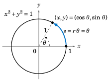
Figure 5.1.1#
The first function we will graph is the sine function. We will describe a geometrical way to create the graph, using the unit circle. This is the circle of radius $1$ in the $xy$-plane consisting of all points $(x,y)$ which satisfy the equation $x^2 + y^2 = 1$ .
We see in Figure 5.1.1 that any point on the unit circle has coordinates \((x,y)=(\cos\;\theta,\sin\;\theta)\), where \(\theta\) is the angle that the line segment from the origin to $(x,y)$ makes with the positive $x$-axis (by definition of sine and cosine). So as the point $(x,y)$ goes around the circle, its $y$-coordinate is \(\sin\;\theta\).
We thus get a correspondence between the $y$-coordinates of points on the unit circle and the values \(f(\theta)=\sin\;\theta\), as shown by the horizontal lines from the unit circle to the graph of \(f(\theta)=\sin\;\theta\) in Figure 5.1.2 for the angles \(\theta = 0\), \(\tfrac{\pi}{6}\), \(\tfrac{\pi}{3}\), \(\tfrac{\pi}{2}\).
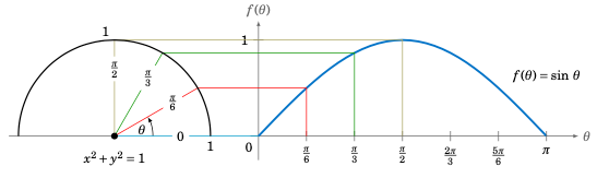
Figure 5.1.2 Graph of sine function based on $y$-coordinate of points on unit circle#
We can extend the above picture to include angles from $0$ to \(2\pi\) radians, as in Figure 5.1.3. This illustrates what is sometimes called the unit circle definition of the sine function.
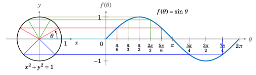
Figure 5.1.3 Unit circle definition of the sine function#
Since the trigonometric functions repeat every \(2\pi\) radians (\(360^\circ\)), we get, for example, the following graph of the function \(y=\sin\;x\) for $x$ in the interval \([-2\pi, 2\pi]\) :
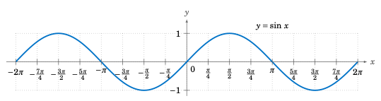
Figure 5.1.4 Graph of \(y=\sin\;x\)#
To graph the cosine function, we could again use the unit circle idea (using the $x$-coordinate of a point that moves around the circle), but there is an easier way. Recall from Section 1.5 that \(\cos\;x = \sin\;(x+90^\circ)\) for all $x$. So \(\cos\;0^\circ\) has the same value as \(\sin\;90^\circ\), \(\cos\;90^\circ\) has the same value as \(\sin\;180^\circ\), \(\cos\;180^\circ\) has the same value as \(\sin\;270^\circ\), and so on. In other words, the graph of the cosine function is just the graph of the sine function shifted to the left by \(90^\circ = \pi/2\) radians, as in Figure 5.1.5:
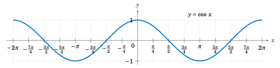
Figure 5.1.5 Graph of \(y=\cos\;x\)#
To graph the tangent function, use \(\tan\;x = \frac{\sin\;x}{\cos\;x}\) to get the following graph:
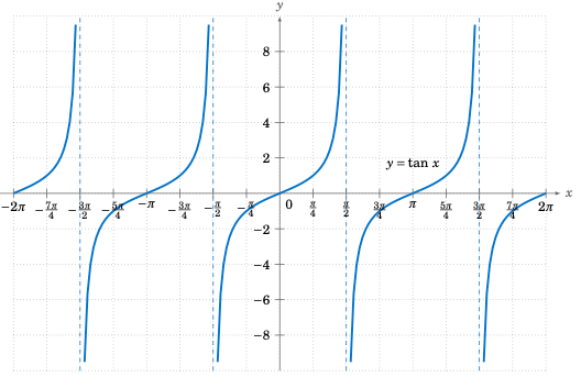
Figure 5.1.6 Graph of \(y=\tan\;x\)#
Recall that the tangent is positive for angles in QI and QIII, and is negative in QII and QIV, and that is indeed what the graph in Figure 5.1.6 shows. We know that \(\tan\;x\) is not defined when \(\cos\;x = 0\), i.e. at odd multiples of \(\frac{\pi}{2}\) : \(x=\pm\,\frac{\pi}{2}\), \(\pm\,\frac{3\pi}{2}\), \(\pm\,\frac{5\pi}{2}\), etc. We can figure out what happens near those angles by looking at the sine and cosine functions. For example, for $x$ in QI near \(\frac{\pi}{2}\), \(\sin\;x\) and \(\cos\;x\) are both positive, with \(\sin\;x\) very close to $1$ and \(\cos\;x\) very close to $0$, so the quotient \(\tan\;x = \frac{\sin\;x}{\cos\;x}\) is a positive number that is very large. And the closer $x$ gets to \(\frac{\pi}{2}\), the larger \(\tan\;x\) gets. Thus, \(x=\frac{\pi}{2}\) is a vertical asymptote of the graph of \(y=\tan\;x\).
Likewise, for $x$ in QII very close to \(\frac{\pi}{2}\), \(\sin\;x\) is very close to $1$ and \(\cos\;x\) is negative and very close to $0$, so the quotient \(\tan\;x = \frac{\sin\;x}{\cos\;x}\) is a negative number that is very large, and it gets larger in the negative direction the closer $x$ gets to \(\frac{\pi}{2}\). The graph shows this. Similarly, we get vertical asymptotes at \(x=-\frac{\pi}{2}\), \(x=\frac{3\pi}{2}\), and \(x=-\frac{3\pi}{2}\), as in Figure 5.1.6. Notice that the graph of the tangent function repeats every \(\pi\) radians, i.e. two times faster than the graphs of sine and cosine repeat.
The graphs of the remaining trigonometric functions can be determined by looking at the graphs of their reciprocal functions. For example, using \(\csc\;x = \frac{1}{\sin\;x}\) we can just look at the graph of \(y=\sin\;x\) and invert the values. We will get vertical asymptotes when \(\sin\;x=0\), namely at multiples of \(\pi\): $x=0$, \(\pm\,\pi\), \(\pm\,2\pi\), etc. Figure 5.1.7 shows the graph of \(y=\csc\;x\), with the graph of \(y=\sin\;x\) (the dashed curve) for reference.
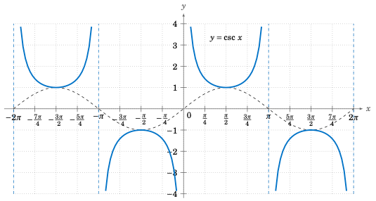
Figure 5.1.7 Graph of \(y=\csc\;x\)#
Likewise, Figure 5.1.8 shows the graph of \(y=\sec\;x\), with the graph of \(y=\cos\;x\) (the dashed curve) for reference. Note the vertical asymptotes at \(x=\pm\,\frac{\pi}{2}\), \(\pm\,\frac{3\pi}{2}\). Notice also that the graph is just the graph of the cosecant function shifted to the left by \(\frac{\pi}{2}\) radians.
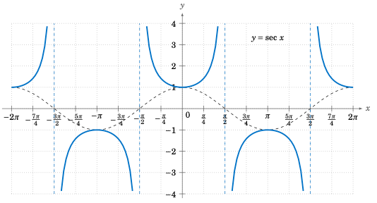
Figure 5.1.8 Graph of \(y=\sec\;x\)#
The graph of \(y=\cot\;x\) can also be determined by using \(\cot\;x = \frac{1}{\tan\;x}\). Alternatively, we can use the relation \(\cot\;x = -\tan\;(x+90^\circ)\) from Section 1.5, so that the graph of the cotangent function is just the graph of the tangent function shifted to the left by \(\frac{\pi}{2}\) radians and then reflected about the $x$-axis, as in Figure 5.1.9:
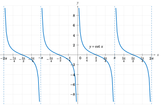
Figure 5.1.9 Graph of \(y=\cot\;x\)#
Example 5.1
Draw the graph of \(y=-\sin\;x\) for \(0 \le x \le 2\pi\).
Solution: Multiplying a function by $-1$ just reflects its graph around the $x$-axis. So reflecting the graph of \(y=\sin\;x\) around the $x$-axis gives us the graph of \(y=-\sin\;x\):
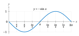
Note that this graph is the same as the graphs of \(y=\sin\;(x \pm \pi)\) and \(y=\cos\;(x+\frac{\pi}{2})\).
It is worthwhile to remember the general shapes of the graphs of the six trigonometric functions, especially for sine, cosine, and tangent. In particular, the graphs of the sine and cosine functions are called sinusoidal curves. Many phenomena in nature exhibit sinusoidal behavior, so recognizing the general shape is important.
Example 5.2
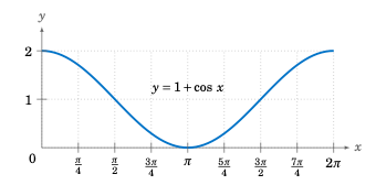
Draw the graph of \(y=1+\cos\;x\) for \(0 \le x \le 2\pi\).
Solution: Adding a constant to a function just moves its graph up or down by that amount, depending on whether the constant is positive or negative, respectively. So adding $1$ to \(\cos\;x\) moves the graph of \(y=\cos\;x\) upward by $1$, giving us the graph of \(y=1+\cos\;x\):
练习#
Exercises
For Exercises 1-12, draw the graph of the given function for \(0 \le x \le 2\pi\).
\(y=-\cos\;x\)
\(y=1+\sin\;x\)
\(y=2-\cos\;x\)
\(y=2-\sin\;x\)
\(y=-\tan\;x\)
\(y=-\cot\;x\)
\(y=1+\sec\;x\)
\(y=-1-\csc\;x\)
\(y=2\sin\;x\)
\(y=-3\cos\;x\)
\(y=-2\tan\;x\)
\(y=-2\sec\;x\)
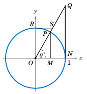
Figure 5.1.10#
We can extend the unit circle definition of the sine and cosine functions to all six trigonometric functions. Let $P$ be a point in QI on the unit circle, so that the line segment \(\overline{OP}\) in Figure 5.1.10 has length $1$ and makes an acute angle \(\theta\) with the positive $x$-axis. Identify each of the six trigonometric functions of \(\theta\) with exactly one of the line segments in Figure 5.1.10, keeping in mind that the radius of the circle is $1$. To get you started, we have \(\sin\;\theta = MP\) (why?).
For Exercise 11, how would you draw the line segments in Figure 5.1.10 if \(\theta\) was in QII? Recall that some of the trigonometric functions are negative in QII, so you will have to come up with a convention for how to treat some of the line segment lengths as negative.
For any point $(x,y)$ on the unit circle and any angle \(\alpha\), show that the point \(R_{\alpha} (x,y)\) defined by \(R_{\alpha} (x,y) = (x\,\cos\;\alpha \,-\, y\,\sin\;\alpha , x\,\sin\;\alpha \,+\, y\,\cos\;\alpha)\) is also on the unit circle. What is the geometric interpretation of \(R_{\alpha} (x,y)\) ? Also, show that \(R_{-\alpha} (R_{\alpha} (x,y)) = (x,y)\) and \(R_{\beta} (R_{\alpha} (x,y)) = R_{\alpha + \beta} (x,y)\).
三角函数图像的性质#
Properties of Graphs of Trigonometric Functions
We saw in Section 5.1 how the graphs of the trigonometric functions repeat every \(2\pi\) radians. In this section we will discuss this and other properties of graphs, especially for the sinusoidal functions (sine and cosine).
First, recall that the domain of a function $f(x)$ is the set of all numbers $x$ for which the function is defined. For example, the domain of \(f(x) = \sin\;x\) is the set of all real numbers, whereas the domain of \(f(x) = \tan\;x\) is the set of all real numbers except \(x=\pm\,\frac{\pi}{2}\), \(\pm\,\frac{3\pi}{2}\), \(\pm\,\frac{5\pi}{2}\), $…$. The range of a function $f(x)$ is the set of all values that $f(x)$ can take over its domain. For example, the range of \(f(x)=\sin\;x\) is the set of all real numbers between $-1$ and $1$ (i.e. the interval \([-1, 1]\)), whereas the range of \(f(x) = \tan\;x\) is the set of all real numbers, as we can see from their graphs.
A function $f(x)$ is periodic if there exists a number $p>0$ such that $x+p$ is in the domain of $f(x)$ whenever $x$ is, and if the following relation holds:
There could be many numbers $p$ that satisfy the above requirements. If there is a smallest such number $p$, then we call that number the period of the function $f(x)$.
Example 5.3
The functions \(\sin\;x\), \(\cos\;x\), $csc;x$, and $sec;x$ all have the same period: \(2\pi\) radians. We saw in Section 5.1 that the graphs of \(y=\tan\;x\) and \(y=\cot\;x\) repeat every \(2\pi\) radians but they also repeat every \(\pi\) radians. Thus, the functions \(\tan\;x\) and \(\cot\;x\) have a period of \(\pi\) radians.
Example 5.4
What is the period of \(f(x)=\sin\;2x\,\)?
Solution: The graph of \(y=\sin\;2x\) is shown in Figure 5.2.1, along with the graph of \(y=\sin\;x\) for comparison, over the interval \([0, 2\pi]\). Note that \(\sin\;2x\) “goes twice as fast” as \(\sin\;x\).
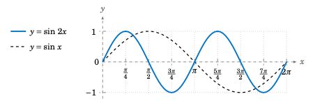
Figure 5.2.1 Graph of \(y=\sin\;2x\)#
For example, for $x$ from $0$ to \(\frac{\pi}{2}\), \(\sin\;x\) goes from $0$ to $1$, but \(\sin\;2x\) is able to go from $0$ to $1$ quicker, just over the interval \([0 , \frac{\pi}{4}]\). While \(\sin\;x\) takes a full \(2\pi\) radians to go through an entire emph{cycle}index{cycle} (the largest part of the graph that does not repeat), \(\sin\;2x\) goes through an entire cycle in just \(\pi\) radians. So the period of \(\sin\;2x\) is \(\pi\) radians.
The above example made use of the graph of \(\sin\;2x\), but the period can be found analytically. Since \(\sin\;x\) has period \(2\pi\), [1] we know that \(\sin\;(x+2\pi) = \sin\;x\) for all $x$. Since $2x$ is a number for all $x$, this means in particular that \(\sin\;(2x+2\pi) = \sin\;2x\) for all $x$. Now define \(f(x)=\sin\;2x\). Then
for all $x$, so the period $p$ of \(\sin\;2x\) is at most \(\pi\), by our definition of period. We have to show that \(p>0\) can not be smaller than \(\pi\). To do this, we will use a proof by contradiction. That is, assume that \(0<p<\pi\), then show that this leads to some contradiction, and hence can not be true. So suppose \(0<p<\pi\). Then \(0<2p<2\pi\), and hence
for all $x$. Since any number $u$ can be written as $2x$ for some $x$ (i.e $u = 2(u/2)$), this means that \(\sin\;u = \sin\;(u+2p)\) for all real numbers $u$, and hence the period of \(\sin\;x\) is as most $2p$. This is a contradiction. Why? Because the period of \(\sin\;x\) is \(2\pi > 2p\). Hence, the period $p$ of \(\sin\;2x\) can not be less than \(\pi\), so the period must equal \(\pi\).
The above may seem like a lot of work to prove something that was visually obvious from the graph (and intuitively obvious by the “twice as fast” idea). Luckily, we do not need to go through all that work for each function, since a similar argument works when \(\sin\;2x\) is replaced by \(\sin\;\omega x\) for any positive real number \(\omega\): instead of dividing \(2\pi\) by $2$ to get the period, divide by \(\omega\). And the argument works for the other trigonometric functions as well. Thus, we get:
For any number \(\omega >0\) :
If \(\omega < 0\), then use \(\sin\;(-A) = -\sin\;A\) and \(\cos\;(-A) = \cos\;A\) (e.g. \(\sin\;(-3x) = -\sin\;3x\)).
Example 5.5
The period of \(y=\cos\;3x\) is \(\frac{2\pi}{3}\) and the period of \(y=\cos\;\frac{1}{2}x\) is \(4\pi\). The graphs of both functions are shown in Figure 5.2.2:
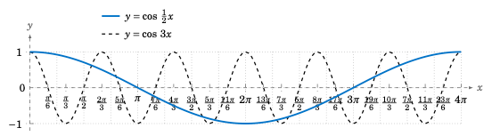
Figure 5.2.2 Graph of \(y=\cos 3x\) and \(y=\cos \frac{1}{2}x\)#
We know that \(\;-1 \le \sin\;x \le 1\;\) and \(\;-1 \le \cos\;x \le 1\;\) for all $x$. Thus, for a constant \(A \ne 0\),
for all $x$. In this case, we call $|A|$ the amplitude of the functions \(y=A\,\sin\;x\) and \(y=A\,\cos\;x\). In general, the amplitude of a periodic curve $f(x)$ is half the difference of the largest and smallest values that $f(x)$ can take:
In other words, the amplitude is the distance from either the top or bottom of the curve to the horizontal line that divides the curve in half, as in Figure 5.2.3.
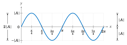
Figure 5.2.3 Amplitude \(= \frac{\text{max} - \text{min}}{2} = \frac{|A| - (-|A|)}{2} = |A|\)#
Not all periodic curves have an amplitude. For example, \(\tan\;x\) has neither a maximum nor a minimum, so its amplitude is undefined. Likewise, \(\cot\;x\), \(\csc\;x\), and \(\sec\;x\) do not have an amplitude. Since the amplitude involves vertical distances, it has no effect on the period of a function, and vice versa.
Example 5.6
Find the amplitude and period of \(y=3\,\cos\;2x\).
Solution: The amplitude is $|3| = 3$ and the period is \(\frac{2\pi}{2}=\pi\). The graph is shown in Figure 5.2.4:
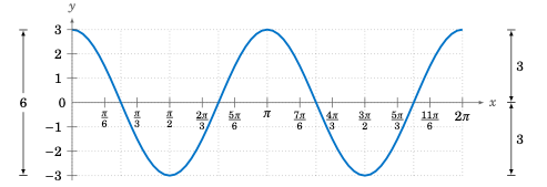
Figure 5.2.4 \(y=3\,\cos\;2x\)#
Example 5.7
Find the amplitude and period of \(y=2 - 3\,\sin\;\frac{2\pi}{3}x\).
Solution: The amplitude of \(-3\,\sin\;\frac{2\pi}{3}x\) is $|-3| =3$. Adding $2$ to that function to get the function \(y=2 - 3\,\sin\;\frac{2\pi}{3}x\) does not change the amplitude, even though it does change the maximum and minimum. It just shifts the entire graph upward by $2$. So in this case, we have
The period is \(\dfrac{2\pi}{\frac{2\pi}{3}}=3\). The graph is shown in Figure 5.2.5:
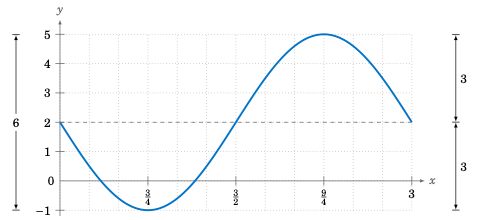
Figure 5.2.5 \(y=2-3\,\sin\;\frac{2\pi}{3}x\)#
Example 5.8
Find the amplitude and period of \(y=2\,\sin\;( x^2 )\).
Solution: This is not a periodic function, since the angle that we are taking the sine of, $x^2$, is not a linear function of $x$, i.e. is not of the form $ax+b$ for some constants $a$ and $b$. Recall how we argued that \(\sin\;2x\) was “twice as fast” as \(\sin\;x\), so that its period was \(\pi\) instead of \(2\pi\). Can we say that \(\sin\;( x^2 )\) is some “constant” times as fast as \(\sin\;x\,\)? No. In fact, we see that the “speed” of the curve keeps increasing as $x$ gets larger, since $x^2$ grows at a variable rate, not a constant rate. This can be seen in the graph of \(y=2\,\sin\;( x^2 )\), shown in Figure 5.2.6: [2]
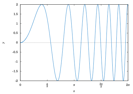
Figure 5.2.6 \(y=2\,\sin\;( x^2 )\)#
Notice how the curve “speeds up” as $x$ gets larger, making the “waves” narrower and narrower. Thus, \(y=2\,\sin\;( x^2 )\) has no period. Despite this, it appears that the function does have an amplitude, namely $2$. To see why, note that since \(|\sin\;\theta| \le 1\) for all \(\theta\), we have
In the exercises you will be asked to find values of $x$ such that \(2\,\sin\;( x^2 )\) reaches the maximum value $2$ and the minimum value $-2$. Thus, the amplitude is indeed $2$. Note: This curve is still sinusoidal despite not being periodic, since the general shape is still that of a “sine wave”, albeit one with variable cycles.
So far in our examples we have been able to determine the amplitudes of sinusoidal curves fairly easily. This will not always be the case.
Example 5.9
Find the amplitude and period of \(y=3\,\sin\;x + 4\,\cos\;x\).
Solution: This is sometimes called a combination sinusoidal curve, since it is the sum of two such curves. The period is still simple to determine: since \(\sin\;x\) and \(\cos\;x\) each repeat every \(2\pi\) radians, then so does the combination \(3\,\sin\;x + 4\,\cos\;x\). Thus, \(y=3\,\sin\;x + 4\,\cos\;x\) has period \(2\pi\). We can see this in the graph, shown in Figure 5.2.7:
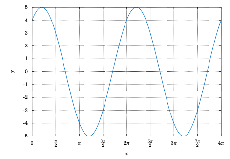
Figure 5.2.7 \(y=3\,\sin\;x + 4\,\cos\;x\)#
The graph suggests that the amplitude is $5$, which may not be immediately obvious just by looking at how the function is defined. In fact, the definition \(y=3\,\sin\;x + 4\,\cos\;x\) may tempt you to think that the amplitude is $7$, since the largest that \(3\,\sin\;x\) could be is $3$ and the largest that \(4\,\cos\;x\) could be is $4$, so that the largest their sum could be is $3+4=7$. However, \(3\,\sin\;x\) can never equal $3$ for the same $x$ that makes \(4\,\cos\;x\) equal to $4$ (why?).
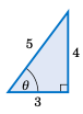
Figure 5.2.8#
There is a useful technique (which we will discuss further in Chapter 6) for showing that the amplitude of \(y=3\,\sin\;x + 4\,\cos\;x\) is $5$. Let \(\theta\) be the angle shown in the right triangle in Figure 5.2.8. Then \(\cos\;\theta = \frac{3}{5}\) and \(\sin\;\theta = \frac{4}{5}\). We can use this as follows:
Thus, \(|y| = |5\,\sin\;(x+\theta)| = |5| \cdot\, |\sin\;(x+\theta)| \le (5)(1) = 5\), so the amplitude of \(y=3\,\sin\;x + 4\,\cos\;x\) is $5$.
In general, a combination of sines and cosines will have a period equal to the lowest common multiple of the periods of the sines and cosines being added. In Example 5.9, \(\sin\;x\) and \(\cos\;x\) each have period \(2\pi\), so the lowest common multiple (which is always an integer multiple) is \(1 \,\cdot\, 2\pi = 2\pi\).
Example 5.10
Find the period of \(y=\cos\;6x + \sin\;4x\).
Solution: The period of \(\cos\;6x\) is \(\frac{2\pi}{6} = \frac{\pi}{3}\), and the period of \(\sin\;4x$ is $\frac{2\pi}{4} = \frac{\pi}{2}\). The lowest common multiple of \(\frac{\pi}{3}\) and \(\frac{\pi}{2}\) is \(\pi\):
Thus, the period of \(y=\cos\;6x + \sin\;4x\) is \(\pi\). We can see this from its graph in Figure 5.2.9:
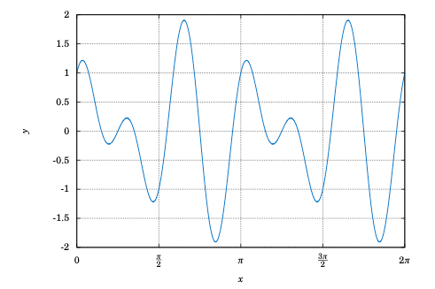
Figure 5.2.9#
What about the amplitude? Unfortunately we can not use the technique from Example 5.9, since we are not taking the cosine and sine of the same angle; we are taking the cosine of $6x$ but the sine of $4x$. In this case, it appears from the graph that the maximum is close to $2$ and the minimum is close to $-2$. In Chapter 6, we will describe how to use a numerical computation program to show that the maximum and minimum are \(\pm\,1.90596111871578\), respectively (accurate to within \(\approx 2.2204 \times 10^{-16}\)). Hence, the amplitude is $1.90596111871578$.
Generalizing Example 5.9, an expression of the form \(a\,\sin\;\omega x \;+\; b\,\cos\;\omega x\) is equivalent to \(\sqrt{a^2 + b^2}\;\sin\;(x+\theta)\), where \(\theta\) is an angle such that \(\cos\;\theta = \frac{a}{\sqrt{a^2 + b^2}}\) and \(\sin\;\theta = \frac{b}{\sqrt{a^2 + b^2}}\). So \(y=a\,\sin\;\omega x \;+\; b\,\cos\;\omega x\) will have amplitude \(\sqrt{a^2 + b^2}\). Note that this method only works when the angle \(\omega x\) is the same in both the sine and cosine terms.
We have seen how adding a constant to a function shifts the entire graph vertically. We will now see how to shift the entire graph of a periodic curve horizontally.
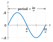
Figure 5.2.10 \(y = A \sin \omega x\)#
Consider a function of the form \(y=A\,\sin\;\omega x\), where $A$ and \(\omega\) are nonzero constants. For simplicity we will assume that $A >0$ and \(\omega > 0\) (in general either one could be negative). Then the amplitude is $A$ and the period is \(\frac{2\pi}{\omega}\). The graph is shown in Figure 5.2.10.
Now consider the function \(y=A\,\sin\;(\omega x - \phi)\), where $phi$ is some constant. The amplitude is still $A$, and the period is still \(\frac{2\pi}{\omega}\), since \(\omega x - \phi\) is a linear function of $x$. Also, we know that the sine function goes through an entire cycle when its angle goes from $0$ to \(2\pi\). Here, we are taking the sine of the angle \(\omega x - \phi\). So as \(\omega x - \phi\) goes from $0$ to \(2\pi\), an entire cycle of the function \(y=A\,\sin\;(\omega x - \phi)\) will be traced out. That cycle starts when
Thus, the graph of \(y=A\,\sin\;(\omega x - \phi)\) is just the graph of \(y=A\,\sin\;\omega x\) shifted horizontally by \(\frac{\phi}{\omega}\), as in Figure 5.2.11. The graph is shifted to the right when \(\phi >0\), and to the left when \(\phi <0\). The amount \(\frac{\phi}{\omega}\) of the shift is called the phase shift of the graph.
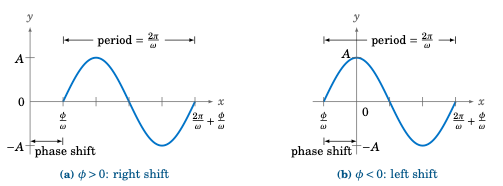
Figure 5.2.11 Phase shift for \(y=A\,\sin\;(\omega x - \phi)\)#
The phase shift is defined similarly for the other trigonometric functions.
Example 5.11
Find the amplitude, period, and phase shift of \(y=3\,\cos\;(2x - \pi)\).
Solution: The amplitude is $3$, the period is \(\frac{2\pi}{2} = \pi\), and the phase shift is \(\frac{\pi}{2}\). The graph is shown in Figure 5.2.12:
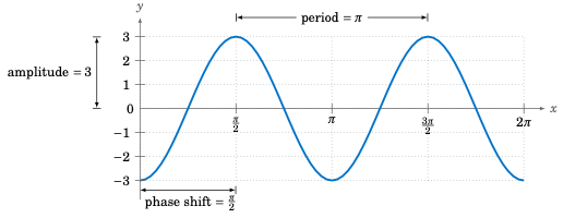
Figure 5.2.12 \(y=3\,\cos\;(2x - \pi)\)#
Notice that the graph is the same as the graph of \(y=3\,\cos\;2x\) shifted to the right by \(\frac{\pi}{2}\), the amount of the phase shift.
Example 5.12
Find the amplitude, period, and phase shift of \(y=-2\,\sin\;\left(3x + \frac{\pi}{2}\right)\).
Solution: The amplitude is $2$, the period is \(\frac{2\pi}{3}\), and the phase shift is \(\frac{-\frac{\pi}{2}}{3} = -\frac{\pi}{6}\). Notice the negative sign in the phase shift, since \(3x+\pi=3x-(-\pi)\) is in the form \(\omega x - \phi\). The graph is shown in Figure 5.2.13:
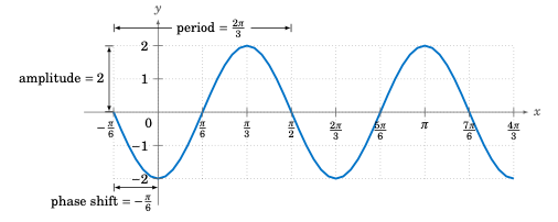
Figure 5.2.13 \(y=-2\,\sin\;\left( 3x + \frac{\pi}{2} \right)\)#
In engineering two periodic functions with the same period are said to be out of phase if their phase shifts differ. For example, \(\sin\;\left( x - \frac{\pi}{6} \right)\) and \(\sin\;x\) would be \(\frac{\pi}{6}\) radians (or \(30^\circ\)) out of phase, and \(\sin\;x\) would be said to lag \(\sin\;\left( x - \frac{\pi}{6} \right)\) by \(\frac{\pi}{6}\) radians, while \(\sin\;\left( x - \frac{\pi}{6} \right)\) leads \(\sin\;x\) by \(\frac{\pi}{6}\) radians. Periodic functions with the same period and the same phase shift are in phase.
The following is a summary of the properties of trigonometric graphs:
For any constants \(A \ne 0\), \(\omega \ne 0\), and \(\phi\):
练习#
Exercises
For Exercises 1-12, find the amplitude, period, and phase shift of the given function. Then graph one cycle of the function, either by hand or by using Gnuplot (see Appendix B).
\(y=3\,\cos\;\pi x\)
\(y=\sin\;(2\pi x - \pi)\)
\(y=-\sin\;(5x + 3)\)
\(y=1+8\,\cos\;(6x- \pi)\)
\(y=2+\cos\;(5x + \pi)\)
\(y=1-\sin\;(3\pi - 2x)\)
\(y=1-\cos\;(3\pi - 2x)\)
\(y=2\,\tan\;(x - 1)\)
\(y=1-\tan\;(3\pi - 2x)\)
\(y=\sec\;(2x + 1)\)
\(y=2\csc\;(2x - 1)\)
\(y=2+4\,\cot\;(1-x)\)
For the function \(y=2\,\sin\;( x^2 )\) in Example 5.8, for which values of $x$ does the function reach its maximum value $2$, and for which values of $x$ does it reach its minimum value
-2?For the function \(y=3\,\sin\;x + 4\,\cos\;x\) in Example 5.9, for which values of $x$ does the function reach its maximum value $5$, and for which values of $x$ does it reach its minimum value
-5? You can restrict your answers to be between $0$ and \(2\pi\).Graph the function \(y=\sin^2 \,x\) from $x=0$ to \(x=2\pi\), either by hand or by using Gnuplot. What are the amplitude and period of this function?
The current \(i(t)\) in an AC electrical circuit at time \(t\ge 0\) is given by \(i(t) = I_m \,\sin\;\omega t\), and the voltage \(v(t)\) is given by \(v(t) = V_m \,\sin\;\omega t\), where \(V_m > I_m > 0\) and \(\omega > 0\) are constants. Sketch one cycle of both \(i(t)\) and \(v(t)\) together on the same graph (i.e. on the same set of axes). Are the current and voltage in phase or out of phase?
Repeat Exercise 16 with \(i(t)\) the same as before but with \(v(t)= V_m \,\sin\;\left(\omega t + \frac{\pi}{4}\right)\).
Repeat Exercise 16 with \(i(t)=-I_m \,\cos\;\left(\omega t - \frac{\pi}{3}\right)\) and \(v(t)= V_m \,\sin\;\left(\omega t - \frac{5\pi}{6}\right)\).
For Exercises 19-21, find the amplitude and period of the given function. Then graph one cycle of the function, either by hand or by using Gnuplot.
\(y=3\,\sin\;\pi x \;-\; 5\,\cos\;\pi x\)
\(y=-5\,\sin\;3x \;+\; 12\,\cos\;3x\)
\(y=2\,\cos\;x \;+\; 2\,\sin\;x\)
Find the amplitude of the function \(y=2\,\sin\;( x^2 ) \;+\; \cos\;( x^2 )\).
For Exercises 23-25, find the period of the given function. Graph one cycle using Gnuplot.
\(y=\sin\;3x \;-\; \cos\;5x\)
\(y=\sin\;\frac{x}{3} \;+\; 2\,\cos\;\frac{3x}{4}\)
\(y=2\,\sin\;\pi x \;+\; 3\,\cos\;\frac{\pi}{3}x\)
Let \(y = 0.5\,\sin\;x ~\sin\;12x\,\). Its graph for $x$ from $0$ to \(4\pi\) is shown in Figure 5.2.14:
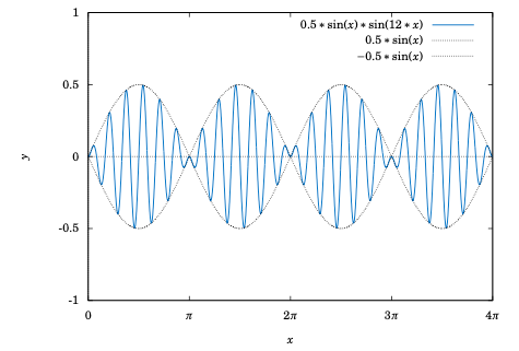
Figure 5.2.14 Modulated wave \(y=0.5\,\sin\;x ~\sin\;12x\)#
You can think of this function as \(\sin\;12x\) with a sinusoidally varying “amplitude” of \(0.5\,\sin\;x\). What is the period of this function? From the graph it looks like the amplitude may be $0.5$. Without finding the exact amplitude, explain why the amplitude is in fact less than $0.5$. The function above is known as a modulated wave, and the functions \(\pm\,0.5\,\sin\;x\) form an amplitude envelope for the wave (i.e. they enclose the wave). Use an identity from Section 3.4 to write this function as a sum of sinusoidal curves.
Use Gnuplot to graph the function \(y= x^2 \,\sin\;10x\) from \(x = -2\pi\) to \(x=2\pi\). What functions form its amplitude envelope? (Note: Use set samples 500 in Gnuplot.)
Use Gnuplot to graph the function \(y= \frac{1}{x^2} \,\sin\;80x\) from $x = 0.2$ to \(x=\pi\). What functions form its amplitude envelope? (Note: Use set samples 500 in Gnuplot.)
Does the function \(y=\sin\;\pi x \;+\; \cos\;x\) have a period? Explain your answer.
Use Gnuplot to graph the function \(y=\frac{\sin\;x}{x}\) from \(x=-4\pi\) to \(x=4\pi\). What happens at $x=0$?
反三角函数#
Inverse Trigonometric Functions
We have briefly mentioned the inverse trigonometric functions before, for example in Section 1.3 when we discussed how to use the \(\boxed{\sin^{-1}}\), \(\boxed{\cos^{-1}}\), and \(\boxed{\tan^{-1}}\) buttons on a calculator to find an angle that has a certain trigonometric function value. We will now define those inverse functions and determine their graphs.
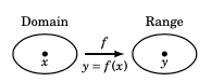
Figure 5.3.1#
Recall that a function is a rule that assigns a single object $y$ from one set (the range) to each object $x$ from another set (the domain). We can write that rule as \(y = f(x)\), where $f$ is the function (see Figure 5.3.1). There is a simple vertical rule for determining whether a rule $y=f(x)$ is a function: $f$ is a function if and only if every vertical line intersects the graph of $y=f(x)$ in the $xy$-coordinate plane at most once (see Figure 5.3.2).
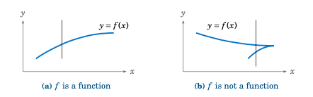
Figure 5.3.2 Vertical rule for functions#
Recall that a function $f$ is one-to-one (often written as $1-1$) if it assigns distinct values of $y$ to distinct values of $x$. In other words, if \(x_1 \ne x_2\) then \(f(x_1 ) \ne f(x_2 )\). Equivalently, $f$ is one-to-one if \(f(x_1 ) = f(x_2 )\) implies \(x_1 = x_2\). There is a simple horizontal rule for determining whether a function $y=f(x)$ is one-to-one: $f$ is one-to-one if and only if every horizontal line intersects the graph of $y=f(x)$ in the $xy$-coordinate plane at most once (see Figure 5.3.3).
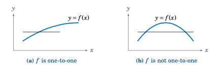
Figure 5.3.3 Horizontal rule for one-to-one functions#
If a function $f$ is one-to-one on its domain, then $f$ has an inverse function, denoted by $f^{-1}$, such that \(y=f(x)\) if and only if \(f^{-1}(y) = x\). The domain of \(f^{-1}\) is the range of $f$.
The basic idea is that $f^{-1}$ “undoes” what $f$ does, and vice versa. In other words,
We know from their graphs that none of the trigonometric functions are one-to-one over their entire domains. However, we can restrict those functions to subsets of their domains where they are one-to-one. For example, \(y=\sin\;x\) is one-to-one over the interval \(\left[ -\frac{\pi}{2},\frac{\pi}{2} \right]\), as we see in the graph below:
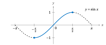
Figure 5.3.4 \(y=\sin\;x\) with $x$ restricted to \(\left[ -\frac{\pi}{2},\frac{\pi}{2} \right]\)#
For \(-\frac{\pi}{2} \le x \le \frac{\pi}{2}\) we have \(-1 \le \sin\;x \le 1\), so we can define the inverse sine function $y=sin^{-1} x$ (sometimes called the arc sine and denoted by \(y=\arcsin\;x\)) whose domain is the interval \([-1, 1]\) and whose range is the interval \(\left[ -\frac{\pi}{2},\frac{\pi}{2} \right]\). In other words:
Example 5.13
Find \(\sin^{-1} \left(\sin\;\frac{\pi}{4}\right)\).
Solution: Since \(-\frac{\pi}{2} \le \frac{\pi}{4} \le \frac{\pi}{2}\), we know that \(\sin^{-1} \left(\sin\;\frac{\pi}{4}\right) = \boxed{\frac{\pi}{4}}\;\), by formula (2).
Example 5.14
Find \(\sin^{-1} \left(\sin\;\frac{5\pi}{4}\right)\).
Solution: Since \(\frac{5\pi}{4} > \frac{\pi}{2}\), we can not use formula (2). But we know that \(\sin\;\frac{5\pi}{4} = -\frac{1}{\sqrt{2}}\). Thus, \(\sin^{-1} \left(\sin\;\frac{5\pi}{4}\right) = \sin^{-1} \left( -\frac{1}{\sqrt{2}} \right)\) is, by definition, the angle $y$ such that \(-\frac{\pi}{2} \le y \le \frac{\pi}{2}\) and \(\sin\;y = -\frac{1}{\sqrt{2}}\). That angle is \(y=-\frac{\pi}{4}\), since
Thus, \(\sin^{-1} \left(\sin\;\frac{5\pi}{4}\right) = \boxed{-\tfrac{\pi}{4}}\;\).
Example 5.14 illustrates an important point: \(\sin^{-1} x\) should always be a number between \(-\frac{\pi}{2}\) and \(\frac{\pi}{2}\). If you get a number outside that range, then you made a mistake somewhere. This why in Example 1.27 in Section 1.5 we got \(\sin^{-1}(-0.682) = -43^\circ\) when using the \(\boxed{\sin^{-1}}\) button on a calculator. Instead of an angle between \(0^\circ\) and \(360^\circ\) (i.e. $0$ to \(2\pi\) radians) we got an angle between \(-90^\circ\) and \(90^\circ\) (i.e. \(-\frac{\pi}{2}\) to \(\frac{\pi}{2}\) radians).
In general, the graph of an inverse function $f^{-1}$ is the reflection of the graph of $f$ around the line $y=x$. The graph of \(y=\sin^{-1} x\) is shown in Figure 5.3.5. Notice the symmetry about the line $y=x$ with the graph of \(y=\sin\;x\).
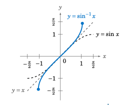
Figure 5.3.5 Graph of \(y=\sin^{-1} x\)#
The inverse cosine function \(y=\cos^{-1} x\) (sometimes called the arc cosine and denoted by \(y=\arccos\;x\)) can be determined in a similar fashion. The function \(y=\cos\;x\) is one-to-one over the interval \([0, \pi]\), as we see in the graph below:
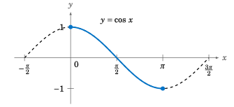
Figure 5.3.6 \(y=\cos\;x\) with $x$ restricted to \([0, \pi]\)#
Thus, \(y=\cos^{-1} x\) is a function whose domain is the interval \([-1, 1]\) and whose range is the interval \([0, \pi]\). In other words:
The graph of \(y=\cos^{-1} x\) is shown below in Figure 5.3.7. Notice the symmetry about the line $y=x$ with the graph of \(y=\cos\;x\).
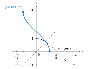
Figure 5.3.7 Graph of \(y=\cos^{-1} x\)#
Example 5.15
Find \(\cos^{-1} \left(\cos\;\frac{\pi}{3}\right)\).
Solution: Since \(0 \le \frac{\pi}{3} \le \pi\), we know that \(\cos^{-1} \left(\cos\;\frac{\pi}{3}\right) = \boxed{\frac{\pi}{3}}\;\), by formula (4).
Example 5.16
Find $cos^{-1} left(cos;frac{4pi}{3}right)$.
Solution: Since \(\frac{4\pi}{3} > \pi\), we can not use formula (4). But we know that \(\cos\;\frac{4\pi}{3} = -\frac{1}{2}\). Thus, \(\cos^{-1} \left(\cos\;\frac{4\pi}{3}\right) = \cos^{-1} \left( -\frac{1}{2} \right)\) is, by definition, the angle $y$ such that \(0 \le y \le \pi\) and \(\cos\;y = -\frac{1}{2}\). That angle is \(y=\frac{2\pi}{3}\) (i.e. \(120^\circ\)). Thus, \(\cos^{-1} \left(\cos\;\frac{4\pi}{3}\right) = \boxed{\tfrac{2\pi}{3}}\;\).
Examples 5.14 and 5.16 may be confusing, since they seem to violate the general rule for inverse functions that \(f^{-1}(f(x)) = x\) for all $x$ in the domain of $f$. But that rule only applies when the function $f$ is one-to-one over its entire domain. We had to restrict the sine and cosine functions to very small subsets of their entire domains in order for those functions to be one-to-one. That general rule, therefore, only holds for $x$ in those small subsets in the case of the inverse sine and inverse cosine.
The inverse tangent function \(y=\tan^{-1} x\) (sometimes called the arc tangent and denoted by \(y=\arctan\;x\)) can be determined similarly. The function \(y=\tan\;x\) is one-to-one over the interval \(\left( -\frac{\pi}{2},\frac{\pi}{2} \right)\), as we see in Figure 5.3.8:
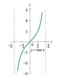
Figure 5.3.8 \(y=\tan\;x\) with $x$ restricted to \(\left( -\frac{\pi}{2},\frac{\pi}{2} \right)\)#
The graph of \(y=\tan^{-1} x\) is shown below in Figure 5.3.9. Notice that the vertical asymptotes for \(y=\tan\;x\) become horizontal asymptotes for \(y=\tan^{-1} x\). Note also the symmetry about the line $y=x$ with the graph of \(y=\tan\;x\).
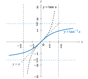
Figure 5.3.9 Graph of \(y=\tan^{-1} x\)#
Thus, \(y=\tan^{-1} x\) is a function whose domain is the set of all real numbers and whose range is the interval \(\left( -\frac{\pi}{2},\frac{\pi}{2} \right)\). In other words:
Example 5.17
Find \(\tan^{-1} \left(\tan\;\frac{\pi}{4}\right)\).
Solution: Since \(-\tfrac{\pi}{2} \le \tfrac{\pi}{4} \le \tfrac{\pi}{2}\), we know that \(\tan^{-1} \left(\tan\;\frac{\pi}{4}\right) = \boxed{\frac{\pi}{4}}\;\), by formula (6).
Example 5.18
Find \(\tan^{-1} \left(\tan\;\pi\right)\).
Solution: Since \(\pi > \tfrac{\pi}{2}\), we can not use formula (6). But we know that \(\tan\;\pi = 0\). Thus, \(\tan^{-1} \left(\tan\;\pi\right) = \tan^{-1} 0\) is, by definition, the angle $y$ such that :mamth:`-\tfrac{\pi}{2} \le y \le \tfrac{\pi}{2}` and \(\tan\;y = 0\). That angle is $y=0$. Thus, \(\tan^{-1} \left(\tan\;\pi \right) = \boxed{0}\;\).
Find the exact value of $cos;left(sin^{-1};left(-frac{1}{4}right)right)$.vspace{1mm}
Example 5.19
Solution: Let \(\theta = \sin^{-1}\;\left(-\frac{1}{4}\right)\). We know that \(-\tfrac{\pi}{2} \le \theta \le \tfrac{\pi}{2}\), so since \(\sin\;\theta = -\frac{1}{4} < 0\), \(\theta\) must be in QIV. Hence \(\cos\;\theta > 0\). Thus,
Note that we took the positive square root above since \(\cos\;\theta > 0\). Thus, \(\cos\;\left(\sin^{-1}\;\left(-\frac{1}{4}\right)\right) = \boxed{\frac{\sqrt{15}}{4}}\;\).
Example 5.20
Show that \(\tan\;(\sin^{-1} x) = \dfrac{x}{\sqrt{1 - x^2}}\) for $-1 < x < 1$.
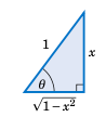
Figure 5.3.10#
Solution: When $x=0$, the formula holds trivially, since
Now suppose that $0 < x < 1$. Let \(\theta = \sin^{-1} x\). Then \(\theta\) is in QI and \(\sin\;\theta = x\). Draw a right triangle with an angle \(\theta\) such that the opposite leg has length $x$ and the hypotenuse has length $1$, as in Figure 5.3.10 (note that this is possible since $0 < x < 1$). Then \(\sin\;\theta = \frac{x}{1} = x\). By the Pythagorean Theorem, the adjacent leg has length \(\sqrt{1 - x^2}\). Thus, \(\tan\;\theta = \frac{x}{\sqrt{1 - x^2}}\).
If $-1 < x < 0$ then \(\theta = \sin^{-1} x\) is in QIV. So we can draw the same triangle except that it would be “upside down” and we would again have \(\tan\;\theta = \frac{x}{\sqrt{1 - x^2}}\), since the tangent and sine have the same sign (negative) in QIV. Thus, \(\tan\;(\sin^{-1} x) = \dfrac{x}{\sqrt{1 - x^2}}\) for $-1 < x < 1$.
The inverse functions for cotangent, cosecant, and secant can be determined by looking at their graphs. For example, the function \(y=\cot\;x\) is one-to-one in the interval \((0,\pi)\), where it has a range equal to the set of all real numbers. Thus, the inverse cotangent \(y=\cot^{-1} x\) is a function whose domain is the set of all real numbers and whose range is the interval \((0,\pi)\). In other words:
The graph of \(y=\cot^{-1} x\) is shown below in Figure 5.3.11.
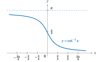
Figure 5.3.11 Graph of \(y=\cot^{-1} x\)#
Similarly, it can be shown that the inverse cosecant \(y=\csc^{-1} x\) is a function whose domain is \(|x| \ge 1\) and whose range is \(-\frac{\pi}{2} \le y \le \frac{\pi}{2}\), \(y \ne 0\). Likewise, the inverse secant \(y=\sec^{-1} x\) is a function whose domain is \(|x| \ge 1\) and whose range is \(0 \le y \le \pi\), \(y \ne \frac{\pi}{2}\).
It is also common to call \(\cot^{-1} x\), \(\csc^{-1} x\), and \(\sec^{-1} x\) the arc cotangent, arc cosecant, and arc secant, respectively, of $x$. The graphs of \(y=\csc^{-1} x\) and \(y=\sec^{-1} x\) are shown in Figure 5.3.12:
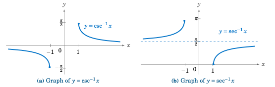
Figure 5.3.12 Graph of \(y=\cot^{-1} x\)#
Example 5.21
Prove the identity $tan^{-1} x ;+; cot^{-1} x ~=~ frac{pi}{2}$.
Solution: Let $theta = cot^{-1} x$. Using relations from Section 1.5, we have
by formula (9). So since \(\tan\;(\tan^{-1} x) = x\) for all $x$, this means that \(\tan\;(\tan^{-1} x) = \tan\;\left( \tfrac{\pi}{2} - \theta \right)\). Thus, \(\tan\;(\tan^{-1} x) = \tan\;\left( \tfrac{\pi}{2} - \cot^{-1} x \right)\). Now, we know that \(0 < \cot^{-1} x < \pi$, so $-\tfrac{\pi}{2} < \tfrac{\pi}{2} - \cot^{-1} x < \tfrac{\pi}{2}\), i.e. \(\tfrac{\pi}{2} - \cot^{-1} x\) is in the restricted subset on which the tangent function is one-to-one. Hence, \(\tan\;(\tan^{-1} x) = \tan\;\left( \tfrac{\pi}{2} - \cot^{-1} x \right)\) implies that \(\tan^{-1} x = \tfrac{\pi}{2} - \cot^{-1} x\), which proves the identity.
Example 5.22
Is $;tan^{-1} a ;+; tan^{-1} b ~=~ tan^{-1} left( dfrac{a+b}{1-ab} right);$ an identity?
Solution: In the tangent addition formula \(\tan\;(A+B) = \dfrac{\tan\;A \;+\; \tan\;B}{1 \;-\; \tan\;A~\tan\;B}\), let \(A = \tan^{-1} a\) and \(B = \tan^{-1} b\). Then
by definition of the inverse tangent. However, recall that \(-\tfrac{\pi}{2} < \tan^{-1} x < \tfrac{\pi}{2}\) for all real numbers $x$. So in particular, we must have \(-\tfrac{\pi}{2} < \tan^{-1} \left( \frac{a+b}{1-ab} \right) < \tfrac{\pi}{2}\). But it is possible that \(\tan^{-1} a \;+\; \tan^{-1} b\) is not in the interval \(\left(-\tfrac{\pi}{2},\tfrac{\pi}{2}\right)\). For example,
And we see that \(\tan^{-1} \left( \frac{1+2}{1-(1)(2)} \right) = \tan^{-1} (-3) = -1.249045 \ne \tan^{-1} 1 \;+\; \tan^{-1} 2\). So the formula is only true when \(-\tfrac{\pi}{2} < \tan^{-1} a \;+\; \tan^{-1} b < \tfrac{\pi}{2}\).
练习#
Exercises
For Exercises 1-25, find the exact value of the given expression in radians.
\(\tan^{-1} 1\)
\(\tan^{-1} \,(-1)\)
\(\tan^{-1} 0\)
\(\cos^{-1} 1\)
\(\cos^{-1} \,(-1)\)
\(\cos^{-1} 0\)
\(\sin^{-1} 1\)
\(\sin^{-1} \,(-1)\)
\(\sin^{-1} 0\)
\(\sin^{-1} \left(\sin\;\frac{\pi}{3}\right)\)
\(\sin^{-1} \left(\sin\;\frac{4\pi}{3}\right)\)
\(\sin^{-1} \left(\sin\;\left(-\frac{5\pi}{6}\right)\right)\)
\(\cos^{-1} \left(\cos\;\frac{\pi}{7}\right)\)
\(\cos^{-1} \left(\cos\;\left(-\frac{\pi}{10}\right)\right)\)
\(\cos^{-1} \left(\cos\;\frac{6\pi}{5}\right)\)
\(\tan^{-1} \left(\tan\;\frac{4\pi}{3}\right)\)
\(\tan^{-1} \left(\tan\;\left(-\frac{5\pi}{6}\right)\right)\)
\(\cot^{-1} \left(\cot\;\frac{4\pi}{3}\right)\)
\(\csc^{-1} \left(\csc\;\left(-\frac{\pi}{9}\right)\right)\)
\(\sec^{-1} \left(\sec\;\frac{6\pi}{5}\right)\)
\(\cos\;\left(\sin^{-1}\;\left(\frac{5}{13}\right)\right)\)
\(\cos\;\left(\sin^{-1}\;\left(-\frac{4}{5}\right)\right)\)
\(\sin^{-1}\;\frac{3}{5} \;+\; \sin^{-1}\;\frac{4}{5}\)
\(\sin^{-1}\;\frac{5}{13} \;+\; \cos^{-1}\;\frac{5}{13}\)
\(\tan^{-1}\;\frac{3}{5} \;+\; \cot^{-1}\;\frac{3}{5}\)
For Exercises 26-33, prove the given identity.
\(\cos\;(\sin^{-1} x) ~=~ \sqrt{1 - x^2}\)
\(\sin\;(\cos^{-1} x) ~=~ \sqrt{1 - x^2}\)
\(\sin^{-1} x \;+\; \cos^{-1} x ~=~ \frac{\pi}{2}\)
\(\sec^{-1} x \;+\; \csc^{-1} x ~=~ \frac{\pi}{2}\)
\(\sin^{-1} (-x) ~=~ -\sin^{-1} x\)
\(\cos^{-1} (-x) \;+\; \cos^{-1} x ~=~ \pi\)
\(\cot^{-1} x ~=~ \tan^{-1} \,\frac{1}{x}~\) for $x>0$
\(\tan^{-1} x \;+\; \tan^{-1} \,\frac{1}{x} ~=~ \frac{\pi}{2}~\) for $x>0$
In Example 5.32 we showed that the formula \(\;\tan^{-1} a \;+\; \tan^{-1} b ~=~ \tan^{-1} \left( \dfrac{a+b}{1-ab} \right)\;\) does not always hold. Does the formula \(\tan\;(\tan^{-1} a \;+\; \tan^{-1} b ) ~=~ \dfrac{a+b}{1-ab}\), which was part of that example, always hold? Explain your answer.
Show that \(\;\tan^{-1}\;\frac{1}{3}\;+\;\tan^{-1}\;\frac{1}{5} ~=~ \tan^{-1}\;\frac{4}{7}\;\).
Show that \(\;\tan^{-1}\;\frac{1}{4}\;+\;\tan^{-1}\;\frac{2}{9} ~=~ \tan^{-1}\;\frac{1}{2}\;\).
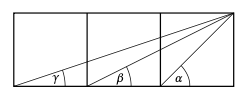
Figure 5.3.13 shows three equal squares lined up against each other. For the angles \(\alpha\), \(\beta\), and \(\gamma\) in the picture, show that \(\alpha = \beta + \gamma\). (Hint: Consider the tangents of the angles.)
Sketch the graph of \(y=\sin^{-1} 2x\).
Write a computer program to solve a triangle in the case where you are given three sides. Your program should read in the three sides as input parameters and print the three angles in degrees as output if a solution exists. Note that since most computer languages use radians for their inverse trigonometric functions, you will likely have to do the conversion from radians to degrees yourself in the program.