第 6 章 附加主题#
Chapter 6 Additional Topics
三角方程的求解#
Solving Trigonometric Equations
An equation involving trigonometric functions is called a trigonometric equation. For example, an equation like
which we encountered in Chapter 1, is a trigonometric equation. In Chapter 1 we were concerned only with finding a single solution (say, between \(0^\circ\) and \(90^\circ\)). In this section we will be concerned with finding the most general solution to such equations.
To see what that means, take the above equation \(\tan\;A = 0.75\). Using the \(\boxed{\tan^{-1}}\) calculator button in degree mode, we get \(A=36.87^\circ\). However, we know that the tangent function has period \(\pi\) rad \(= 180^\circ\), i.e. it repeats every \(180^\circ\). Thus, there are many other possible answers for the value of \(A\), namely \(36.87^\circ + 180^\circ\), \(36.87^\circ - 180^\circ\), \(36.87^\circ + 360^\circ\), \(36.87^\circ - 360^\circ\), \(36.87^\circ + 540^\circ\), etc. We can write this in a more compact form:
This is the most general solution to the equation. Often the part that says \(\text{for }k=0, \pm\,1, \pm\,2, ...\) is omitted since it is usually understood that k varies over all integers. The general solution in radians would be:
Example 6.1
Solve the equation \(\;2\,\sin\;\theta \;+\;1 ~=~ 0\).
Solution: Isolating \(\sin\;\theta\) gives \(\;\sin\;\theta ~=~ -\tfrac{1}{2}\). Using the \(\boxed{\sin^{-1}}\) calculator button in degree mode gives us \(\theta = -30^\circ\), which is in QIV. Recall that the reflection of this angle around the \(y\)-axis into QIII also has the same sine. That is, \(\sin\;210^\circ = -\tfrac{1}{2}\). Thus, since the sine function has period \(2\pi\) rad \(= 360^\circ\), and since \(-30^\circ\) does not differ from \(210^\circ\) by an integer multiple of \(360^\circ\), the general solution is:
In radians, the solution is:
For the rest of this section we will write our solutions in radians.
Example 6.2
Solve the equation \(\;2\cos^2 \;\theta \;-\; 1 ~=~ 0\).
Solution: Isolating \(\;\cos^2 \;\theta\) gives us
and since the period of cosine is \(2\pi\), we would add \(2\pi k\) to each of those angles to get the general solution. But notice that the above angles differ by multiples of \(\frac{\pi}{2}\). So since every multiple of 2pi is also a multiple of \(\frac{\pi}{2}\), we can combine those four separate answers into one:
Example 6.3
Solve the equation \(\;2\,\sec\;\theta ~=~ 1\).
Solution: Isolating \(\;\sec\;\theta\) gives us
which is impossible. Thus, there is fbox{no solution};.
Example 6.4
Solve the equation \(\;\cos\;\theta ~=~ \tan\;\theta\).
Solution: The idea here is to use identities to put everything in terms of a single trigonometric function:
The last equation looks more complicated than the original equation, but notice that it is actually a quadratic equation: making the substitution \(x=\sin\;\theta\), we have
by the quadratic formula from elementary algebra. But \(-1.618 < -1\), so it is impossible that \(\;\sin\theta = x = -1.618\). Thus, we must have \(\;\sin\;\theta = x = 0.618\). Hence, there are two possible solutions: \(\theta = 0.666 ` rad in QI and its reflection :math:\)pi - theta = 2.475` rad around the \(y\)-axis in QII. Adding multiples of \(2\pi\) to these gives us the general solution:
Example 6.5
Solve the equation ;sin;theta ~=~ tan;theta.
Solution: Trying the same method as in the previous example, we get
plus multiples of \(2\pi\). So since the above angles are multiples of \(\pi\), and every multiple of \(2\pi\) is a multiple of \(\pi\), we can combine the two answers into one for the general solution:
Example 6.6
Solve the equation \(\;\cos\;3\theta ~=~ \frac{1}{2}\).
Solution: The idea here is to solve for \(3\theta\) first, using the most general solution, and then divide that solution by \(3\). So since \(\;\cos^{-1} \frac{1}{2} = \frac{\pi}{3}\), there are two possible solutions for \(3\theta\): 3theta = frac{pi}{3} in QI and its reflection \(-3\theta = -\frac{\pi}{3}\) around the \(x\)-axis in QIV. Adding multiples of \(2\pi\) to these gives us:
Example 6.7
Solve the equation \(\;\sin\;2\theta ~=~ \sin\;\theta\).
Solution: Here we use the double-angle formula for sine:
Example 6.8
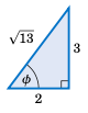
Figure 6.1.1#
Solve the equation \(\;2\,\sin\;\theta \;-\; 3\,\cos\;\theta ~=~ 1\).
Solution: We will use the technique which we discussed in \(Chapter 5 <c5>\) for finding the amplitude of a combination of sine and cosine functions. Take the coefficients \(2\) and \(3\) of \(\;\sin\;\theta\) and \(\;-\cos\;\theta\), respectively, in the above equation and make them the legs of a right triangle, as in Figure 6.1.1. Let \(\phi\) be the angle shown in the right triangle. The leg with length \(3 >0\) means that the angle \(\phi\) is above the \(x\)-axis, and the leg with length \(2>0\) means that \(\phi\) is to the right of the \(y\)-axis. Hence, \(\phi\) must be in QI. The hypotenuse has length \(\sqrt{13}\) by the Pythagorean Theorem, and hence \(\;\cos\;\phi = \frac{2}{\sqrt{13}}\) and \(\;\sin\;\theta = \frac{3}{\sqrt{13}}\). We can use this to transform the equation to solve as follows:
Now, since \(\;\cos\;\phi = \frac{2}{\sqrt{13}}\) and \(\phi\) is in QI, the most general solution for \(\phi\) is \(\phi = 0.983 + 2\pi k\) for \(k=0\), \(\pm\,1\), \(\pm\,2\), \(...\) . So since we needed to add multiples of \(2\pi\) to the solutions \(0.281\) and \(2.861\) anyway, the most general solution for \(\theta\) is:
Note: In Example 6.8 if the equation had been \(\;2\,\sin\;\theta \;+\; 3\,\cos\;\theta ~=~ 1\) then we still would have used a right triangle with legs of lengths 2 and 3, but we would have used the sine addition formula instead of the subtraction formula.
练习#
Exercises
For Exercises 1-12, solve the given equation (in radians).
\(\tan\;\theta \;+\; 1 ~=~ 0\)
\(2\,\cos\;\theta \;+\; 1 ~=~ 0\)
\(\sin\;5\theta \;+\; 1 ~=~ 0\)
\(2\,\cos^2 \;\theta \;-\; \sin^2 \;\theta ~=~ 1\)
\(2\,\sin^2 \;\theta \;-\; \cos\;2\theta ~=~ 0\)
\(2\,\cos^2 \;\theta \;+\; 3\,\sin\;\theta ~=~ 0\)
\(\cos^2 \;\theta \;+\; 2\,\sin\;\theta ~=~ -1\)
\(\tan\;\theta \;+\; \cot\;\theta ~=~ 2\)
\(\sin\;\theta ~=~ \cos\;\theta\)
\(2\,\sin\;\theta \;-\; 3\,\cos\;\theta ~=~ 0\)
\(\cos^2 \;3\theta \;-\; 5\,\cos\;3\theta \;+\; 4 ~=~ 0\)
\(3\,\sin\;\theta \;-\; 4\,\cos\;\theta ~=~ 1\)
三角学中的数值方法#
Numerical Methods in Trigonometry
We were able to solve the trigonometric equations in the previous section fairly easily, which in general is not the case. For example, consider the equation
There is a solution, as shown in Figure 6.2.1 below. The graphs of \(y=\cos\;x\) and \(y=x\) intersect somewhere between \(x=0\) and \(x=1\), which means that there is an \(x\) in the interval \([0, 1]\) such that \(\cos\;x = x\).
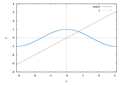
Figure 6.2.1 \(y=\cos\;x\) and \(y=x\)#
Unfortunately there is no trigonometric identity or simple method which will help us here. Instead, we have to resort to numerical methods, which provide ways of getting successively better approximations to the actual solution(s) to within any desired degree of accuracy. There is a large field of mathematics devoted to this subject called numerical analysis. Many of the methods require calculus, but luckily there is a method which we can use that requires just basic algebra. It is called the secant method, and it finds roots of a given function \(f(x)\), i.e. values of \(x\) such that \(f(x)=0\). A derivation of the secant method is beyond the scope of this book, [1] but we can state the algorithm it uses to solve \(f(x)=0\):
Pick initial points \(x_0\) and \(x_1\) such that \(x_0 < x_1\) and \(f(x_0)\,f(x_1) < 0\) (i.e. the solution is somewhere between \(x_0\) and \(x_1\)).
For \(n \ge 2\), define the number \(x_n\) by
(2)#\[x_n ~=~ x_{n-1} ~-~ \dfrac{(x_{n-1} \;-\; x_{n-2})\,f(x_{n-1})}{f(x_{n-1}) \;-\; f(x_{n-2})}\]as long as \(|x_{n-1} \;-\; x_{n-2}| > \epsilon_{error}\), where \(\epsilon_{error} > 0\) is the maximum amount of error desired (usually a very small number).
The numbers \(x_0\), \(x_1\), \(x_2\), \(x_3\), \(...\) will approach the solution \(x\) as we go through more iterations, getting as close as desired.
We will now show how to use this algorithm to solve the equation \(\cos\;x = x\). The solution to that equation is the root of the function \(f(x) =\cos\;x - x\). And we saw that the solution is somewhere in the interval \([0, 1]\) . So pick \(x_0 = 0\) and \(x_1 = 1\). Then \(f(0)=1\) and \(f(1)=-0.4597\), so that \(f(x_0)\,f(x_1) < 0\) (we are using radians, of course). Then by definition,
and so on. Using a calculator is not very efficient and will lead to rounding errors. A better way to implement the algorithm is with a computer. Listing 6.1 below shows the code (secant.java) for solving \(\cos\;x = x\) with the secant method, using the Java programming language:
Listing 6.1 Program listing for secant.java
 1import java.math.*;
 2public class secant {
 3public static void main (String[] args) {
 4    double x0 =  Double.parseDouble(args[0]);
 5    double x1 =  Double.parseDouble(args[1]);
 6    double x = 0;
 7    double error = 1.0E-50;
 8    for (int i=2; i <= 10; i++) {
 9        if (Double.compare(Math.abs(x0 - x1),error) > 0) {
10          x = x1 - (x1 - x0)*f(x1)/(f(x1) - f(x0));
11          x0 = x1;
12          x1 = x;
13          System.out.println("x" + i + " = " + x);
14        } else {
15          break;
16        }
17    }
18    MathContext mc = new MathContext(50);
19    BigDecimal answer = new BigDecimal(x,mc);
20    System.out.println("x = " + answer);
21  }
22  //Define the function f(x)
23  public static double f (double x) {
24    return Math.cos(x) - x;
25  }
26}
Lines 4-5 read in \(x_0\) and \(x_1\) as input parameters to the program.
Line 6 initializes the variable that will eventually hold the solution.
Line 7 sets the maximum error \(\epsilon_{error}\) to be \(1.0 \,\times\, 10^{-50}\). That is, our final answer will be within that (tiny!) amount of the real solution.
Line 8 starts a loop of 9 iterations of the algorithm, i.e. it will create the successive approximations \(x_2\), \(x_3\), \(...\), \(x_{10}\) to the real solution, though in Line 9 we check to see if the two previous approximations differ by less than the maximum error. If they do, we stop (since this means we have an acceptable solution), otherwise we continue.
Line 10 is the main step in the algorithm, creating \(x_n\) from \(x_{n-1}\) and \(x_{n-2}\).
Lines 11-12 set the new values of \(x_{n-2}\) and \(x_{n-1}\), respectively.
Lines 18-20 set the number of decimal places to show in the final answer to 50 (the default is 16) and then print the answer.
Lines 23-24 give the definition of the function \(f(x)=\cos\;x - x\).
Below is the result of compiling and running the program using \(x_0 = 0\) and \(x_1 = 1\):
javac secant.java
java secant 0 1
x2 = 0.6850733573260451
x3 = 0.736298997613654
x4 = 0.7391193619116293
x5 = 0.7390851121274639
x6 = 0.7390851332150012
x7 = 0.7390851332151607
x8 = 0.7390851332151607
x = 0.73908513321516067229310920083662495017051696777344
Notice that the program only got up to \(x_8\), not \(x_{10}\). The reason is that the difference between \(x_8\) and \(x_7\) was small enough (less than \(\epsilon_{error} = 1.0 \,\times\, 10^{-50}\)) to stop at \(x_8\) and call that our solution. The last line shows that solution to 50 decimal places.
Does that number look familiar? It should, since it is the answer to Exercise 11 in Section 4.1. That is, when taking repeated cosines starting with any number (in radians), you eventually start getting the above number repeatedly after enough iterations. This turns out not to be a coincidence. Figure 6.2.2 gives an idea of why.
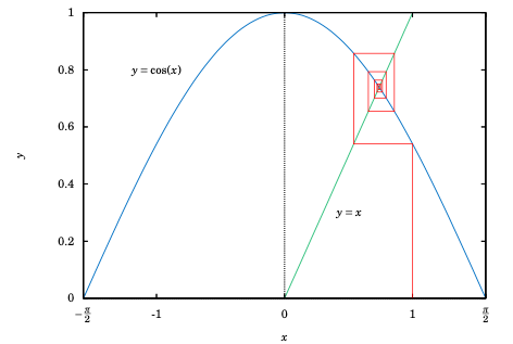
Figure 6.2.2 Attractive fixed point for \(\cos\;x\)#
Since \(x=0.73908513321516...\) is the solution of \(\cos\;x = x\), you would get \(\cos\;(\cos\;x) = \cos\;x = x\), so \(\cos\;(\cos\;(\cos\;x)) = \cos\;x = x\), and so on. This number \(x\) is called an attractive fixed point of the function \(\cos\;x\). No matter where you start, you end up getting “drawn” to it. Figure 6.2.2 shows what happens when starting at \(x=0\): taking the cosine of 0 takes you to 1, and then successive cosines (indicated by the intersections of the vertical lines with the cosine curve) eventually “spiral” in a rectangular fashion to the fixed point (i.e. the solution), which is the intersection of \(y=\cos\;x\) and \(y=x\).
Recall in Example 5.10 in Section 5.2 that we claimed that the maximum and minimum of the function \(y=\cos\;6x + \sin\;4x\) were \(\pm\,1.90596111871578\), respectively. We can show this by using the open-source program Octave. [2] Octave uses a successive quadratic programming method to find the minimum of a function \(f(x)\). Finding the maximum of \(f(x)\) is the same as finding the minimum of \(-f(x)\) then multiplying by \(-1\) (why?). Below we show the commands to run at the Octave command prompt (octave:n>) to find the minimum of \(f(x) = \cos\;6x + \sin\;4x\). The command sqp(3,'f') says to use \(x=3\) as a first approximation of the number x where f(x) is a minimum.
octave:1> format long
octave:2> function y = f(x)
> y = cos(6*x) + sin(4*x)
> endfunction
octave:3> sqp(3,'f')
y = -1.90596111871578
ans = 2.65792064609274
The output says that the minimum occurs when \(x=2.65792064609274\) and that the minimum is \(-1.90596111871578\). To find the maximum of \(f(x)\), we find the minimum of -f(x) and then take its negative. The command sqp(2,'f') says to use x=2 as a first approximation of the number \(x\) where \(f(x)\) is a maximum.
octave:4> function y = f(x)
> y = -cos(6*x) - sin(4*x)
> endfunction
octave:5> sqp(2,'f')
y = -1.90596111871578
ans = 2.05446832062993
The output says that the maximum occurs when x=2.05446832062993 and that the maximum is -(-1.90596111871578) = 1.90596111871578.
Recall from Section 2.4 that Heron’s formula is adequate for “typical” triangles, but will often have a problem when used in a calculator with, say, a triangle with two sides whose sum is barely larger than the third side. However, you can get around this problem by using computer software capable of handling numbers with a high degree of precision. Most modern computer programming languages have this capability. For example, in the Python programming language [3] (chosen here for simplicity) the decimal module can be used to set any level of precision. [4] Below we show how to get accuracy up to 50 decimal places using Heron’s formula for the triangle in Example 2.16 from Section 2.4, by using the python interactive command shell:
>>> from decimal import *
>>> getcontext().prec = 50
>>> a = Decimal("1000000")
>>> b = Decimal("999999.9999979")
>>> c = Decimal("0.0000029")
>>> s = (a+b+c)/2
>>> K = s*(s-a)*(s-b)*(s-c)
>>> print Decimal(K).sqrt()
0.99999999999894999999999894874999999889618749999829
(Note: The triple arrow >>> is just a command prompt, not part of the code.)
Notice in this case that we do get the correct answer; the high level of precision eliminates the rounding errors shown by many calculators when using Heron’s formula.
Another software option is Sage [5], a powerful and free open-source mathematics package based on Python. It can be run on your own computer, but it can also be run through a web interface: go to http://sagenb.org to create a free account, then once you register and sign in, click the New Worksheet link to start entering commands. For example, to find the solution to \(\cos\;x = x\) in the interval \([0, 1]\) , enter these commands in the worksheet textfield:
x = var('x')
find_root(cos(x) == x, 0,1)
Click the evaluate link to display the answer: 0.7390851332151559
练习#
Exercises
One obvious solution to the equation \(2\,\sin\;x = x\) is \(x=0\). Write a program to find the other solution(s), accurate to at least within \(1.0 \,\times\, 10^{-20}\). You can use any programming language, though you may find it easier to just modify the code in Listing 6.1 (only one line needs to be changed!). It may help to use Gnuplot to get an idea of where the graphs of \(y=2\,\sin\;x\) and \(y=x\) intersect.
Repeat Exercise 1 for the equation \(\sin\;x = x^2\).
Use Octave or some other program to find the maximum and minimum of \(y=\cos\;5x - \sin\;3x\).
复数#
Complex Numbers
There is no real number x such that \(x^2 = -1\). However, it turns out to be useful [6] to invent such a number, called the imaginary unit and denoted by the letter i. Thus, \(i^2 = -1\), and hence \(i = \sqrt{-1}\). If a and b are real numbers, then a number of the form \(a + bi\) is called a complex number, and if \(b \ne 0\) then it is called an imaginary number (and pure imaginary if a=0 and \(b \ne 0\)). The real number a is called the real part of the complex number a+bi, and bi is called its imaginary part.
What does it mean to add a to bi in the definition a+bi of a complex number, i.e. adding a real number and an imaginary number? You can think of it as a way of extending the set of real numbers. If b=0 then \(a+bi = a+0i = a\) (since 0i is defined as 0), so that every real number is a complex number.
The imaginary part bi in \(a+bi\) can be thought of as a way of taking the one-dimensional set of all real numbers and extending it to a two-dimensional set: there is a natural correspondence between a complex number \(a+bi\) and a point \((a,b)\) in the (two-dimensional) \(xy\)-coordinate plane.
Before exploring that correspondence further, we will first state some fundamental properties of and operations on complex numbers:
Let a+bi and c+di be complex numbers. Then:
\(a+bi ~=~ c+di\) if and only if
a=candb=d~(i.e. the real parts are equal and the imaginary parts are equal)\((a+bi) \;+\; (c+di) ~=~ (a+c) \;+\; (b+d)i~\) (i.e. add the real parts together and add the imaginary parts together)
\((a+bi) \;-\; (c+di) ~=~ (a-c) \;+\; (b-d)i\)
\((a+bi)\,(c+di) ~=~ (ac-bd) \;+\; (ad+bc)i\)
\((a+bi)\,(a-bi) ~=~ a^2 \;+\; b^2\)
\(\dfrac{a+bi}{c+di} ~=~ \dfrac{(ac+bd) \;+\; (bc-ad)i}{c^2 + d^2}\)
The first three items above are just definitions of equality, addition, and subtraction of complex numbers. The last three items can be derived by treating the multiplication and division of complex numbers as you would normally treat factors of real numbers:
The fifth item is a special case of the multiplication formula:
The sixth item comes from using the previous items:
The conjugate \(\overline{a+bi}\) of a complex number a+bi is defined as \(\overline{a+bi} = a-bi\). Notice that \((a+bi) \;+\; \overline{(a+bi)} ~=~ 2a\) is a real number, \((a+bi) \;-\; \overline{(a+bi)} ~=~ 2bi\) is an imaginary number if \(b \ne 0\), and \((a+bi) \overline{(a+bi)} ~=~ a^2 + b^2\) is a real number. So for a complex number \(z=a+bi\), \(z\,\overline{z} = a^2 + b^2 \,\) and thus we can define the modulus of z to be \(\sqrt{z\,\overline{z}} = \sqrt{a^2 + b^2}\), which we denote by \(|z|\).
Example 6.9
Let \(z_1 = -2+3i\) and \(z_2 = 3+4i\). Find \(z_1 + z_2\), \(z_1 - z_2\), \(z_1 \, z_2\), \(z_1 / z_2\), \(|z_1|\), and \(|z_2|\).
Solution: Using our rules and definitions, we have:
We know that any point \((x,y)\) in the \(xy\)-coordinate plane that is a distance \(r >0\) from the origin has coordinates \(x=r\,\cos\;\theta\) and \(y=r\,\sin\;\theta\), where \(\theta\) is the angle in standard position as in Figure 6.3.1 (a).
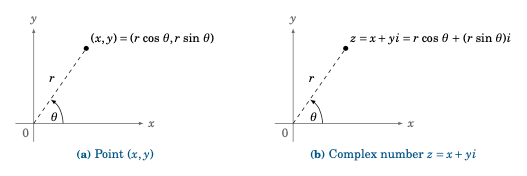
Figure 6.3.1#
Let \(z=x+yi\) be a complex number. We can represent z as a point in the complex plane, where the horizontal \(x\)-axis represents the real part of z, and the vertical \(y\)-axis represents the pure imaginary part of z, as in Figure 6.3.1 (b). The distance r from z to the origin is, by the Pythagorean Theorem, \(r = \sqrt{x^2 + y^2}\), which is just the modulus of z. And we see from Figure 6.3.1 (b) that \(x=r\,\cos\;\theta\) and \(y=r\,\sin\;\theta\), where \(\theta\) is the angle formed by the positive \(x\)-axis and the line segment from the origin to z. We call this angle \(\theta\) the argument of z. Thus, we get the trigonometric form (sometimes called the polar form) of the complex number z:
小技巧
For any complex number \(z=x+yi\), we can write
The representation \(z=r\,(\cos\;\theta \;+\; i\,\sin\;\theta)\) is often abbreviated as:
In the special case \(z=0 = 0+0i\), the argument \(\theta\) is undefined since \(r=|z|=0\). Also, note that the argument \(\theta\) can be replaced by \(\theta \;+\; 360^\circ k\) or \(\theta \;+\; \pi k\), depending on whether you are using degrees or radians, respectively, for \(k=0\), \(\pm\,1\), \(\pm\,2\), \(...\) . Note also that for \(z=x+yi\) with \(r=|z|\), \(\theta\) must satisfy
Example 6.10
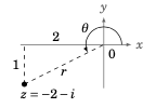
Figure 6.3.2#
Represent the complex number \(-2 - i\) in trigonometric form.
Solution: Let \(z=-2-i=x+yi\), so that \(x=-2\) and \(y=-1\). Then \(\theta\) is in QIII, as we see in Figure 6.3.2. So since \(\tan\;\theta = \tfrac{y}{x} = \tfrac{-1}{-2} = \tfrac{1}{2}\), we have \(\theta = 206.6^\circ\). Also,
Thus, \(\boxed{-2 - i = \sqrt{5}\;(\cos\;206.6^\circ \;+\; i\,\sin\;206.6^\circ)}\;\), or \(\sqrt{5}\;\text{cis}\;206.6^\circ\).
For complex numbers in trigonometric form, we have the following formulas for multiplication and division:
小技巧
Let \(z_1 = r_1 \,(\cos\;\theta_1 \;+\; i\,\sin\;\theta_1 )\) and \(z_2 = r_2 \,(\cos\;\theta_2 \;+\; i\,\sin\;\theta_2 )\) be complex numbers. Then
The proofs of these formulas are straightforward:
by the addition formulas for sine and cosine. And
by the subtraction formulas for sine and cosine, and since \(\cos^2 \,\theta_2 \;+\;\sin^2 \,\theta_2 = 1\). [.qed]
Note that formulas (5) and (6) say that when multiplying complex numbers the moduli are multiplied and the arguments are added, while when dividing complex numbers the moduli are divided and the arguments are subtracted. This makes working with complex numbers in trigonometric form fairly simple.
Example 6.11
Let \(z_1 = 6\,(\cos\;70^\circ \;+\; i\,\sin\;70^\circ )\) and \(z_1 = 2\,(\cos\;31^\circ \;+\; i\,\sin\;31^\circ )\). Find \(z_1 \, z_2\) and \(\frac{z_1}{z_2}\).
Solution: By formulas (5) and (6) we have
For the special case when \(z_1 = z_2 = z = r\,(\cos\;\theta \;+\; i\,\sin\;\theta)\) in formula (5), we have
and so
and continuing like this (i.e. by mathematical induction), we get:
We define \(z^0 = 1\) and \(z^{-n} = 1/z^n\) for all integers \(n \ge 1\). So by De Moivre’s Theorem and formula (5), for any \(z=r\,(\cos\;\theta \;+\; i\,\sin\;\theta)\) and integer \(n \ge 1\) we get
and so De Moivre’s Theorem in fact holds for all integers. [8]
Example 6.12
Find \((1+i)^{10}\).
Solution: Since \(1+i = \sqrt{2}\;(\cos\;45^\circ \;+\; i\,\sin\;45^\circ )\) (why?), by De Moivre’s Theorem we have
We can use De Moivre’s Theorem to find the \(n^{th}\) roots of a complex number. That is, given any complex number z and positive integer n, find all complex numbers w such that \(w^n = z\). Let \(z=r\,(\cos\;\theta \;+\; i\,\sin\;\theta)\). Since the cosine and sine functions repeat every \(360^\circ\), we know that \(z=r\,(\cos\;(\theta + 360^\circ k)\;+\; i\,\sin\;(\theta + 360^\circ k))\) for \(k=0\), \(\pm\,1\), \(\pm\,2\), \(...\). Now let \(w=r_0 \,(\cos\;\theta_0 \;+\; i\,\sin\;\theta_0 )\) be an \(n^{th}\) root of z. Then
Since the cosine and sine of \(\frac{\theta + 360^\circ k}{n}\) will repeat for \(k \ge n\), we get the following formula for the \(n^{th}\) roots of z:
小技巧
For any nonzero complex number \(z=r\,(\cos\;\theta \;+\; i\,\sin\;\theta)\) and positive integer n, the n distinct \(n^{th}\)
roots of z are
for \(k=0\), 1, 2, …, n-1.
Note: An \(n^{th}\) root of z is usually written as \(z^{1/n}\) or \(\sqrt[n]{z}\). The number \(r^{1/n}\) in the above formula is the usual real n^{th} root of the real number \(r=|z|\).
Example 6.13:
Find the three cube roots of i.
Solution: Since \(i = 1\,(\cos\;90^\circ \;+\; i\,\sin\;90^\circ)\), the three cube roots of i are:
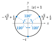
Figure 6.3.3#
Notice from Example 6.13 that the three cube roots of i are equally spaced points along the unit circle \(|z|=1\) in the complex plane, as shown in Figure 6.3.3. We see that consecutive cube roots are \(120^\circ\) apart.
In general, the \(n\) \(n^{th}\) roots of a complex number z will be equally spaced points along the circle of radius \(|z|^{1/n}\) in the complex plane, with consecutive roots separated by \(\tfrac{360^\circ}{n}\).
In higher mathematics the Fundamental Theorem of Algebra states that every polynomial of degree n with complex coefficients has n complex roots (some of which may repeat). In particular, every real number a has \(n\) n^{th} roots (being the roots of \(z^n - a\)). For example, the square roots of 1 are \(\pm\,1\), and the square roots of -1 are \(\pm\,i\).
练习#
Exercises
For Exercises 1-16, calculate the given expression.
\((2+3i) \;+\; (-3-2i)\)
\((2+3i) \;-\; (-3-2i)\)
\((2+3i) \;\cdot\; (-3-2i)\)
\((2+3i)/(-3-2i)\)
\(\overline{(2+3i)} \;+\; \overline{(-3-2i)}\)
\(\overline{(2+3i)} \;-\; \overline{(-3-2i)}\)
\((1+i)/(1-i)\)
\(|-3+2i|\)
\(i^3\)
\(i^4\)
\(i^5\)
\(i^6\)
\(i^7\)
\(i^8\)
\(i^9\)
\(i^{2009}\)
For Exercises 17-24, prove the given identity for all complex numbers.
\(\overline{\left( \overline{z} \right)} \;=\; z\)
\(\overline{z_1 + z_2} \;=\; \overline{z_1} + \overline{z_2}\)
\(\overline{z_1 - z_2} \;=\; \overline{z_1} - \overline{z_2}\)
\(\overline{z_1 \, z_2} \;=\; \overline{z_1} ~ \overline{z_2}\)
\(\overline{\left( \dfrac{z_1}{z_2} \right)} \;=\; \dfrac{\overline{z_1}}{\overline{z_2}}\)
\(|z| \;=\; |\overline{z}|\phantom{\dfrac{|1_1|}{|1_2|}}\)
\(|z_1 \, z_2| \;=\; |z_1|\,|z_2|\phantom{\dfrac{|1_1|}{|1_2|}}\)
\(\left| \dfrac{z_1}{z_2} \right| \;=\; \dfrac{|z_1|}{|z_2|}\)
For Exercises 25-30, put the given number in trigonometric form.
\(2+3i\)
\(-3-2i\)
\(1-i\)
\(-i\)
\(1\)
\(-1\)
Verify that De Moivre’s Theorem holds for the power \(n=0\).
For Exercises 32-35, calculate the given number.
\(3\,(\cos\;14^\circ \;+\; i\,\sin\;14^\circ ) \;\cdot\; 2\,(\cos\;121^\circ \;+\; i\,\sin\;121^\circ )\)
\(\lbrack 3\,(\cos\;14^\circ \;+\; i\,\sin\;14^\circ )\rbrack^4\phantom{\dfrac{3}{4}}\)
\(\lbrack 3\,(\cos\;14^\circ \;+\; i\,\sin\;14^\circ )\rbrack^{-4}\phantom{\dfrac{3}{4}}\)
\(\dfrac{3\,(\cos\;14^\circ \;+\; i\,\sin\;14^\circ )}{ 2\,(\cos\;121^\circ \;+\; i\,\sin\;121^\circ )}\)
Find the three cube roots of \(-i\).
Find the three cube roots of \(1+i\).
Find the three cube roots of \(1\).
Find the three cube roots of \(-1\).
Find the five fifth roots of \(1\).
Find the five fifth roots of \(-1\).
Find the two square roots of \(-2 + 2\sqrt{3}\,i\).
Prove that if \(z\) is an \(n^{th}\) root of a real number
a, then so is \(\overline{z}\). (Hint: Use Exercise 20.)
极坐标#
Polar Coordinates
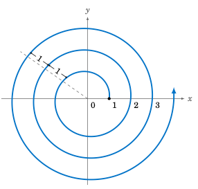
Figure 6.4.1#
Suppose that from the point \((1,0)\) in the \(xy\)-coordinate plane we draw a spiral around the origin, such that the distance between any two points separated by \(360^\circ\) along the spiral is always 1, as in Figure 6.4.1. We can not express this spiral as \(y=f(x)\) for some function f in Cartesian coordinates, since its graph violates the vertical rule.
However, this spiral would be simple to describe using the polar coordinate system. Recall that any point P distinct from the origin (denoted by O) in the \(xy\)-coordinate plane is a distance r>0 from the origin, and the ray \(\overrightarrow{OP}\) makes an angle \(\theta\) with the positive \(x\)-axis, as in Figure ref{fig:polar}. We call the pair \((r,\theta)\) the polar coordinates of P, and the positive \(x\)-axis is called the polar axis of this coordinate system. Note that \((r,\theta) = (r,\theta + 360^\circ k)\) for \(k=0\), \(\pm\,1\), \(\pm\,2\), \(...\), so (unlike for Cartesian coordinates) the polar coordinates of a point are not unique.
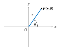
Figure 6.4.2 Polar coordinates \((r,\theta)\)#
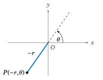
Figure 6.4.3 Negative r: \((-r,\theta)\)#
In polar coordinates we adopt the convention that r can be negative, by defining \((-r,\theta) = (r,\theta + 180^\circ)\) for any angle \(\theta\). That is, the ray \(\overrightarrow{OP}\) is drawn in the opposite direction from the angle \(\theta\), as in Figure 6.4.3. When \(r=0\), the point \((r,\theta) = (0,\theta)\) is the origin O, regardless of the value of \(\theta\).
You may be familiar with graphing paper, for plotting points or functions given in Cartesian coordinates (sometimes also called rectangular coordinates). Such paper consists of a rectangular grid. Similar graphing paper exists for plotting points and functions in polar coordinates, similar to Figure 6.4.4.
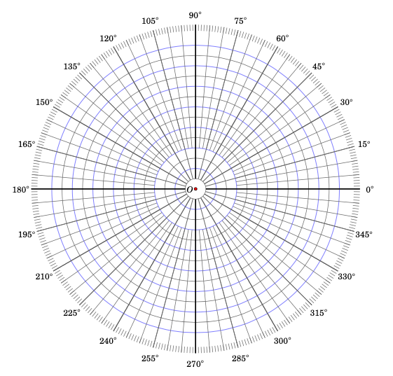
Figure 6.4.4 Polar coordinate graph#
The angle \(\theta\) can be given in either degrees or radians, whichever is more convenient. Radians are often preferred when graphing functions in polar coordinates. The reason is that, unlike degrees, radians can be considered “unitless” (as we mentioned in Chapter 4). This is desirable when a function given in polar coordinates is expressed as r as a function of \(\theta\) (similar to how, in Cartesian coordinates \((x,y)\), functions are usually expressed as y as a function of x). For example, if a function in polar coordinates is written as \(r = 2\,\theta\), then r would have the same units as \(\theta\). But r should be a unitless quantity, hence using radians for \(\theta\) makes more sense in this case.
Example6.14
Express the spiral from Figure 6.4.1 in polar coordinates.
Solution: We will use radians for theta. The goal is to find some equation involving r and \(\theta\) that describes the spiral. We see that
for \(k=0,1,2,\ldots\). In fact, that last relation holds for any nonnegative real number k (why?). So for any \(\theta \ge 0\),
Hence, the spiral can be written as \(\boxed{r ~=~ 1 + \frac{\theta}{2\pi}}\) for \(\theta \ge 0\). The graph is shown in Figure 6.4.5, along with the Gnuplot commands to create the graph.
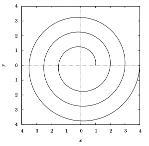
Figure 6.4.5 \(r = 1 + \frac{\theta}{2\pi}\)#
set polar
set size square
set samples 2000
unset key
set zeroaxis
set xlabel "x"
set ylabel "y"
plot [0:6*pi] 1 + t/(2*pi)
Note that when using the set polar command, Gnuplot will assume that the function being plotted is r as a function of \(\theta\) (represented by the variable t in Gnuplot).
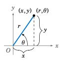
Figure 6.4.6#
Figure 6.4.6 shows how to convert between polar coordinates and Cartesian coordinates. For a point with polar coordinates \((r,\theta)\) and Cartesian coordinates \((x,y)\):
- Polar to Cartesian:
- (9)#\[\boxed{ x ~=~ r\,\cos\;\theta \qquad y ~=~ r\,\sin\;\theta }\]
- Cartesian to Polar:
- (10)#\[\boxed{ r ~=~ \pm\;\sqrt{x^2 ~+~ y^2} \qquad \tan\;\theta ~=~ \frac{y}{x} ~~\text{if `x \ne 0`} }\]
Note that in formula 6.10, if \(x = 0\) then \(\theta = \pi/2\) or \(\theta = 3\pi/2\). Also, if \(x \ne 0\) and \(y \ne 0\) then the two possible solutions for \(\theta\) in the equation \(\tan\;\theta ~=~ \frac{y}{x}\) are in opposite quadrants (for \(0 \le \theta < 2\pi\)). If the angle \(\theta\) is in the same quadrant as the point \((x,y)\), then \(r = \sqrt{x^2 ~+~ y^2}\) (i.e. r is positive); otherwise \(r = -\sqrt{x^2 ~+~ y^2}\) (i.e. r is negative).
Example 6.15
Convert the following points from polar coordinates to Cartesian coordinates:
(a) \((2,30^\circ)\); (b) \((3,3\pi/4)\); (c) \((-1,5\pi/3)\)
Solution:
(a) Using formula 6.9 with \(r=2\) and \(\theta = 30^\circ\), we get:
(b) Using formula 6.9 with \(r=3\) and \(\theta = 3\pi/4\), we get:
(c) Using formula 6.9 with \(r=-1\) and \(\theta = 5\pi/3\), we get:
Example 6.16
Convert the following points from Cartesian coordinates to polar coordinates:
(a) (3,4); (b) (-5,-5)
Solution:
(a) Using formula 6.10 with x=3 and y=4, we get:
Since \(\theta = 53.13^\circ\) is in the same quadrant (QI) as the point \((x,y) = (3,4)\), we can take \(r ~=~ \sqrt{x^2 + y^2} = \sqrt{3^2 + 4^2} = 5\). Thus, :math:`boxed{(r,theta) = (5,53.13^circ)}`~.
Note that if we had used \(\theta = 233.13^\circ\), then we would have \((r,\theta) = (-5,233.13^\circ)\).
(b) Using formula 6.10 with x=-5 and y=-5, we get:
Since \(\theta = 225^\circ\) is in the same quadrant (QIII) as the point \((x,y) = (-5,-5)\), we can take \(r ~=~ \sqrt{x^2 + y^2} = \sqrt{(-5)^2 + (-5)^2} = 5\,\sqrt{2}\). Thus, :math:`boxed{(r,theta) = (5,sqrt{2},225^circ)}`~.
Note that if we had used \(\theta = 45^\circ\), then we would have \((r,\theta) = (-5\,\sqrt{2},45^\circ)\).
Example 6.17
Write the equation \(x^2 + y^2 = 9\) in polar coordinates.
Solution: This is just the equation of a circle of radius 3 centered at the origin. Since \(r = \pm\sqrt{x^2 + y^2} = \pm\sqrt{9}\), in polar coordinates the equation can be written as simply :math:`boxed{r = 3}`~.
Example 6.18
Write the equation x^2 + (y-4)^2 = 16 in polar coordinates.
Solution: This is the equation of a circle of radius 4 centered at the point (0,4). Expanding the equation, we get:
Why could we cancel r from both sides in the last step? Because the point (0,0) is on the circle, canceling r does not eliminate r=0 as a potential solution of the equation (since \(\theta = 0^\circ\) would make \(r = 8\,\sin\;\theta = 8\,\sin\;0^\circ = 0\)). Thus, the equation is :math:`boxed{r = 8,sin;theta}`~.
Example 6.19
Write the equation \(y = x\) in polar coordinates.
Solution: This is the equation of a line through the origin. So when \(x=0\), we know that \(y=0\). When \(x \ne 0\), we get:
Since there is no restriction on r, we could have r=0 and \(\theta = 45^\circ\), which would take care of the case \(x = 0\) (since then \((x,y) = (0,0)\), which is the same as \((r,\theta) = (0,45^\circ))\). Thus, the equation is \(\boxed{\theta = 45^\circ}~\).
Example 6.20
Prove that the distance d between two points \((r_1 , \theta_1)\) and \((r_2 , \theta_2)\) in polar coordinates is
Solution: The idea here is to use the distance formula in Cartesian coordinates, then convert that to polar coordinates. So write
Then \((x_1,y_1)\) and \((x_2,y_2)\) are the Cartesian equivalents of \((r_1 , \theta_1)\) and \((r_2 , \theta_2)\), respectively. Thus, by the Cartesian coordinate distance formula,
so the result follows by taking square roots of both sides.
In Example 6.17 we saw that the equation \(x^2 + y^2 = 9\) in Cartesian coordinates could be expressed as \(r = 3\) in polar coordinates. This equation describes a circle centered at the origin, so the circle is symmetric about the origin. In general, polar coordinates are useful in situations when there is symmetry about the origin (though there are other situations), which arise in many physical applications.
练习#
Exercises
For Exercises 1-5, convert the given point from polar coordinates to Cartesian coordinates.
\((6,210^\circ)\)
\((-4,3\pi)\)
\((2,11\pi/6)\)
\((6,90^\circ)\)
\((-1,405^\circ)\)
For Exercises 6-10, convert the given point from Cartesian coordinates to polar coordinates.
6. \((3,1)\) 8. \((-1,-3)\) 9. \((0,2)\) 10. \((4,-2)\) 11. \((-2,0)\)
For Exercises 11-18, write the given equation in polar coordinates.
\((x-3)^2 + y^2 = 9\)
\(y = -x\)
\(x^2 - y^2 = 1\)
\(3x^2 + 4y^2 - 6x = 9\)
Graph the function \(r = 1 + 2\,\cos\;\theta\) in polar coordinates.