更改基准和投影#
Changing datums and projections
如果您还记得,在 第 2 章 GIS 中,我们讨论了 基准 是地球形状的数学模型,而 投影 是将地球表面上的点转换为二维地图上的点的一种方式。有大量可用的基准和投影 - 无论何时处理地理空间数据,您都必须知道您的数据使用哪个基准和哪个投影(如果有)。如果您要组合来自多个来源的数据,您通常必须将地理空间数据从一个基准更改为另一个基准,或从一个投影更改为另一个投影。
If you remember, in Chapter 2, GIS, we discussed that a datum is a mathematical model of the Earth’s shape, while a projection is a way of translating points on the Earth’s surface into points on a two-dimensional map. There are a large number of available datums and projections—whenever you are working with geospatial data, you must know which datum and which projection (if any) your data uses. If you are combining data from multiple sources, you will often have to change your geospatial data from one datum to another, or from one projection to another.
任务 – 更改投影以使用地理和 UTM 坐标合并 Shapefile#
Task – change projections to combine shapefiles using geographic and UTM coordinates
在这个示例中,我们将处理两个具有不同投影的 shapefile。我们还没有遇到使用投影的地理空间数据——迄今为止我们看到的所有数据都使用了地理(未投影的)纬度和经度值。因此,首先我们将下载一些 通用横轴墨卡托(UTM) 投影的地理空间数据。
WebGIS 网站(http://webgis.com)提供了描述土地利用和土地覆盖的 shapefile,称为 LULC 数据文件。对于这个示例,我们将下载一个关于佛罗里达州南部(具体来说是戴德县)的 shapefile,该文件使用了通用横轴墨卡托投影。
您可以从以下 URL 下载该 shapefile:
http://webgis.com/MAPS/fl/lulcutm/miami.zip
解压后的目录包含了 shapefile 文件,名为 miami.shp,以及一个 datum_reference.txt 文件,描述了该 shapefile 的坐标系统。该文件告诉我们以下内容:
LULC shapefile 是由 Lakes Environmental Software 从原始的 USGS GIRAS LULC 文件生成的。
基准面:NAD83
投影:UTM
区域:17
美国地质调查局(USGS)数据收集日期:1972年
参考: http://edcwww.cr.usgs.gov/products/landcover/lulc.html
因此,这个特定的 shapefile 使用 UTM 区域 17 投影,基准面为 NAD83。
现在让我们来看第二个 shapefile,这次使用的是地理坐标。我们将使用 GSHHS 海岸线数据库,它使用 WGS84 基准面和地理(纬度/经度)坐标。
备注
您不需要为此示例下载 GSHHS 数据库;虽然我们将显示一个将 LULC 数据覆盖在 GSHHS 数据之上的地图,您只需要 LULC shapefile 即可完成这个食谱。绘制类似本示例中展示的地图将会在 第8章:使用 Python 和 Mapnik 绘制地图 中讲解。
我们不能直接比较这两个 shapefile 中的坐标;LULC shapefile 的坐标是以 UTM(即从给定参考线起的米数)为单位,而 GSHHS shapefile 的坐标则是以纬度和经度值(十进制度)为单位:
备注
- LULC: x=485719.47, y=2783420.62
x=485779.49, y=2783380.63 x=486129.65, y=2783010.66 …
- GSHHS: x=180.0000, y=68.9938
x=180.0000, y=65.0338 x=179.9984, y=65.0337
在我们可以将这两个 shapefile 合并之前,我们必须首先将它们转换为使用相同的投影。我们将通过将 LULC shapefile 从 UTM-17 转换为地理(纬度/经度)坐标来实现这一点。为此,我们需要定义一个 坐标转换,然后将该转换应用于 shapefile 中的每个特征。
下面是如何使用 OGR 定义坐标转换:
from osgeo import osr

srcProjection = osr.SpatialReference()
srcProjection.SetUTM(17)

dstProjection = osr.SpatialReference()
dstProjection.SetWellKnownGeogCS('WGS84') # Lat/long.

transform = osr.CoordinateTransformation(srcProjection,
                                       dstProjection)
使用此转换,我们可以将 shapefile 中的每个特征从 UTM 投影转换为地理坐标:
for i in range(layer.GetFeatureCount()):
      feature = layer.GetFeature(i)
      geometry = feature.GetGeometryRef()
      geometry.Transform(transform)
将所有这些与我们之前探索的技术结合起来,通过将特征从一个 shapefile 复制到另一个 shapefile,我们将得到以下完整程序:
# changeProjection.py

import os, os.path, shutil
from osgeo import ogr
from osgeo import osr
from osgeo import gdal

# 定义源投影和目标投影,以及用于转换的转换对象。

srcProjection = osr.SpatialReference()
srcProjection.SetUTM(17)

dstProjection = osr.SpatialReference()
dstProjection.SetWellKnownGeogCS('WGS84') # Lat/long.

transform = osr.CoordinateTransformation(srcProjection,
                                          dstProjection)

# 打开源 shapefile。

srcFile = ogr.Open("miami/miami.shp")
srcLayer = srcFile.GetLayer(0)

# 创建目标 shapefile,并赋予新的投影。

if os.path.exists("miami-reprojected"):
      shutil.rmtree("miami-reprojected")
os.mkdir("miami-reprojected")

driver = ogr.GetDriverByName("ESRI Shapefile")
dstPath = os.path.join("miami-reprojected", "miami.shp")
dstFile = driver.CreateDataSource(dstPath)
dstLayer = dstFile.CreateLayer("layer", dstProjection)

# 逐个重投影每个特征。

for i in range(srcLayer.GetFeatureCount()):
      feature = srcLayer.GetFeature(i)
      geometry = feature.GetGeometryRef()

      newGeometry = geometry.Clone()
      newGeometry.Transform(transform)

      feature = ogr.Feature(dstLayer.GetLayerDefn())
      feature.SetGeometry(newGeometry)
      dstLayer.CreateFeature(feature)
      feature.Destroy()

# 完成。

srcFile.Destroy()
dstFile.Destroy()
备注
注意,本示例并未将字段值复制到新的 shapefile 中;如果您的 shapefile 含有元数据,您需要在创建每个新特征时将字段复制过来。另外,上述代码假设 miami.shp shapefile 已经被放置在 miami 子目录中;如果您将该 shapefile 存储在其他位置,您需要修改 ogr.Open() 语句以使用正确的路径名。
在运行此程序处理 miami.shp shapefile 后,shapefile 中所有特征的坐标将从 UTM-17 转换为地理坐标:
重投影前:  x=485719.47, y=2783420.62
            x=485779.49, y=2783380.63
            x=486129.65, y=2783010.66
            ...

重投影后:  x=-81.1417, y=25.1668
            x=-81.1411, y=25.1664
            x=-81.1376, y=25.1631
为了验证这个过程是否成功,让我们绘制一张地图,显示重投影后的 LULC 数据与 GSHHS 海岸线数据的叠加:
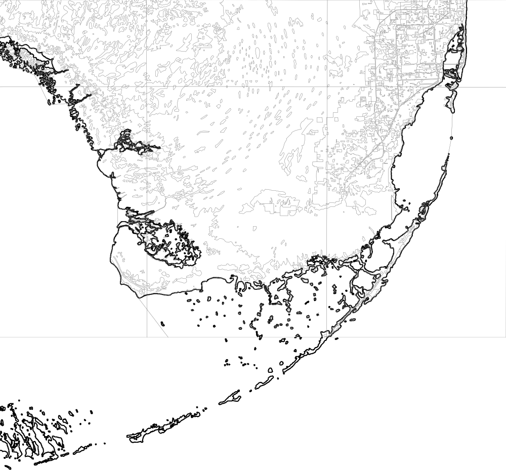
浅灰色轮廓显示了 LULC shapefile 中的各个多边形,而黑色轮廓显示了由 GLOBE shapefile 定义的海岸线。现在,这两个 shapefile 都使用地理坐标,正如您所看到的,海岸线完全匹配。
备注
如果您仔细观察,可能会注意到 LULC 数据使用的是 NAD83 基准面,而 GSHHS 数据和我们重投影后的 LULC 数据都使用的是 WGS84 基准面。我们可以这样做而不会出错,因为这两个基准面在北美地区的点是相同的。
In this recipe, we will work with two shapefiles that have different projections. We haven’t yet encountered any geospatial data that uses a projection—all the data we’ve seen so far uses geographic (unprojected) latitude and longitude values. So let’s start by downloading some geospatial data in Universal Transverse Mercator (UTM) projection.
The WebGIS website (http://webgis.com) provides shapefiles describing land-use and land-cover, called LULC datafiles. For this example, we will download a shapefile for southern Florida (Dade County, to be exact), which uses the Universal Transverse Mercator projection.
You can download this shapefile from the following URL:
http://webgis.com/MAPS/fl/lulcutm/miami.zip
The decompressed directory contains the shapefile, called miami.shp, along with a datum_reference.txt file describing the shapefile’s coordinate system. This file tells us the following:
The LULC shape file was generated from the original USGS GIRAS LULC
file by Lakes Environmental Software.
Datum: NAD83
Projection: UTM
Zone: 17
Data collection date by U.S.G.S.: 1972
Reference: http://edcwww.cr.usgs.gov/products/landcover/lulc.html
So this particular shapefile uses UTM Zone 17 projection, and a datum of NAD83.
Let’s take a second shapefile, this time in geographic coordinates. We’ll use the GSHHS shoreline database, which uses the WGS84 datum and geographic (latitude/longitude) coordinates.
备注
You don’t need to download the GSHHS database for this example; while we will display a map overlaying the LULC data on top of the GSHHS data, you only need the LULC shapefile to complete this recipe. Drawing maps such as the one shown in this recipe will be covered in Chapter 8, Using Python and Mapnik to Produce Maps.
We can’t directly compare the coordinates in these two shapefiles; the LULC shapefile has coordinates measured in UTM (that is, in meters from a given reference line), while the GSHHS shapefile has coordinates in latitude and longitude values (in decimal degrees):
备注
- LULC: x=485719.47, y=2783420.62
x=485779.49, y=2783380.63 x=486129.65, y=2783010.66 …
- GSHHS: x=180.0000, y=68.9938
x=180.0000, y=65.0338 x=179.9984, y=65.0337
Before we can combine these two shapefiles, we first have to convert them to use the same projection. We’ll do this by converting the LULC shapefile from UTM-17 to geographic (latitude/longitude) coordinates. Doing this requires us to define a coordinate transformation and then apply that transformation to each of the features in the shapefile.
Here is how you can define a coordinate transformation using OGR:
from osgeo import osr

srcProjection = osr.SpatialReference()
srcProjection.SetUTM(17)

dstProjection = osr.SpatialReference()
dstProjection.SetWellKnownGeogCS('WGS84') # Lat/long.

transform = osr.CoordinateTransformation(srcProjection,
                                       dstProjection)
Using this transformation, we can transform each of the features in the shapefile from UTM projection back into geographic coordinates:
for i in range(layer.GetFeatureCount()):
    feature = layer.GetFeature(i)
    geometry = feature.GetGeometryRef()
    geometry.Transform(transform)
Putting all this together with the techniques we explored earlier for copying the features from one shapefile to another, we end up with the following complete program:
# changeProjection.py

import os, os.path, shutil
from osgeo import ogr
from osgeo import osr
from osgeo import gdal

# Define the source and destination projections, and a
# transformation object to convert from one to the other.

srcProjection = osr.SpatialReference()
srcProjection.SetUTM(17)

dstProjection = osr.SpatialReference()
dstProjection.SetWellKnownGeogCS('WGS84') # Lat/long.

transform = osr.CoordinateTransformation(srcProjection,
                                         dstProjection)

# Open the source shapefile.

srcFile = ogr.Open("miami/miami.shp")
srcLayer = srcFile.GetLayer(0)

# Create the dest shapefile, and give it the new projection.

if os.path.exists("miami-reprojected"):
    shutil.rmtree("miami-reprojected")
os.mkdir("miami-reprojected")

driver = ogr.GetDriverByName("ESRI Shapefile")
dstPath = os.path.join("miami-reprojected", "miami.shp")
dstFile = driver.CreateDataSource(dstPath)
dstLayer = dstFile.CreateLayer("layer", dstProjection)

# Reproject each feature in turn.

for i in range(srcLayer.GetFeatureCount()):
    feature = srcLayer.GetFeature(i)
    geometry = feature.GetGeometryRef()

    newGeometry = geometry.Clone()
    newGeometry.Transform(transform)

    feature = ogr.Feature(dstLayer.GetLayerDefn())
    feature.SetGeometry(newGeometry)
    dstLayer.CreateFeature(feature)
    feature.Destroy()

# All done.

srcFile.Destroy()
dstFile.Destroy()
备注
Note that this example doesn’t copy field values into the new shapefile; if your shapefile has metadata, you will want to copy the fields across as you create each new feature. Also, the preceding code assumes that the miami.shp shapefile has been placed into a miami sub-directory; you’ll need to change the ogr.Open() statement to use the appropriate path name if you’ve stored this shapefile in a different place.
After running this program over the miami.shp shapefile, the coordinates for all the features in the shapefile will have been converted from UTM-17 into geographic coordinates:
Before reprojection:  x=485719.47, y=2783420.62
                      x=485779.49, y=2783380.63
                      x=486129.65, y=2783010.66
                      ...

After reprojection:   x=-81.1417, y=25.1668
                      x=-81.1411, y=25.1664
                      x=-81.1376, y=25.1631
To see whether this worked, let’s draw a map showing the reprojected LULC data overlaid on the GSHHS shoreline data:
The light gray outlines show the various polygons within the LULC shapefile, while the black outline shows the shoreline as defined by the GLOBE shapefile. Both of these shapefiles now use geographic coordinates, and as you can see the coastlines match exactly.
备注
If you have been watching closely, you may have noticed that the LULC data is using the NAD83 datum, while the GSHHS data and our reprojected version of the LULC data both use the WGS84 datum. We can do this without error because the two datums are identical for points within North America.
任务 – 更改基准以允许合并较旧和较新的 TIGER 数据#
Task – change datums to allow older and newer TIGER data to be combined
在这个示例中,我们需要获取一些使用 NAD27 基准面的地理空间数据。该基准面起源于 1927 年,并在 1980 年代之前广泛用于北美的地理空间分析,随后被 NAD83 替代。
ESRI 提供了一套从 2000 年美国人口普查中转换为 shapefile 格式的 TIGER/Line 文件。这些文件可以从以下链接下载:
http://esri.com/data/download/census2000-tigerline/index.html
对于 2000 年的人口普查数据,除了阿拉斯加使用较旧的 NAD27 基准面外,其他所有 TIGER/Line 文件都使用 NAD83。因此,我们可以使用前面提到的网站下载包含 NAD27 基准面特征的 shapefile。访问该网站,点击 Preview and Download 超链接,然后从下拉菜单中选择 Alaska。选择 Line Features - Roads 图层,然后点击 Submit Selection 按钮。
这些数据按县进行划分。勾选 Anchorage 旁边的复选框,然后点击 Proceed to Download 按钮,下载包含安克雷奇道路详细信息的 shapefile。下载后的 shapefile 文件名为 tgr02020lkA.shp,并保存在名为 lkA02020 的目录中。
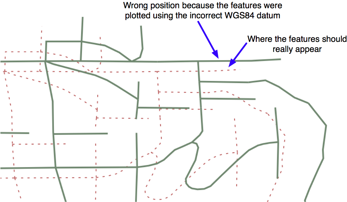
如网站所述,该数据使用的是 NAD27 基准面。如果我们假设该 shapefile 使用的是 WSG83 基准面,所有特征将会出现在错误的位置:
为了使特征出现在正确的位置,并且能够将这些特征与使用 WGS84 基准面的其他数据合并,我们需要将 shapefile 转换为 WGS84。将 shapefile 从一个基准面转换到另一个基准面需要与我们之前用来从一个投影转换到另一个投影的相同基本过程:首先选择源基准面和目标基准面,并定义一个坐标转换来进行转换:
srcDatum = osr.SpatialReference()
srcDatum.SetWellKnownGeogCS('NAD27')

dstDatum = osr.SpatialReference()
dstDatum.SetWellKnownGeogCS('WGS84')

transform = osr.CoordinateTransformation(srcDatum, dstDatum)
然后,您可以处理 shapefile 中的每个特征,使用坐标转换转换特征的几何形状:
for i in range(srcLayer.GetFeatureCount()):
   feature = srcLayer.GetFeature(i)
   geometry = feature.GetGeometryRef()
   geometry.Transform(transform)
下面是完整的 Python 程序,用于将 lkA02020 shapefile 从 NAD27 基准面转换为 WGS84:
# changeDatum.py

import os, os.path, shutil
from osgeo import ogr
from osgeo import osr
from osgeo import gdal

# 定义源基准面和目标基准面,以及一个
# 转换对象来进行转换。

srcDatum = osr.SpatialReference()
srcDatum.SetWellKnownGeogCS('NAD27')

dstDatum = osr.SpatialReference()
dstDatum.SetWellKnownGeogCS('WGS84')

transform = osr.CoordinateTransformation(srcDatum, dstDatum)

# 打开源 shapefile。

srcFile = ogr.Open("lkA02020/tgr02020lkA.shp")
srcLayer = srcFile.GetLayer(0)

# 创建目标 shapefile,并赋予新的投影。

if os.path.exists("lkA-reprojected"):
   shutil.rmtree("lkA-reprojected")
os.mkdir("lkA-reprojected")

driver = ogr.GetDriverByName("ESRI Shapefile")
dstPath = os.path.join("lkA-reprojected", "lkA02020.shp")
dstFile = driver.CreateDataSource(dstPath)
dstLayer = dstFile.CreateLayer("layer", dstDatum)

# 逐个重投影每个特征。

for i in range(srcLayer.GetFeatureCount()):
   feature = srcLayer.GetFeature(i)
   geometry = feature.GetGeometryRef()
   newGeometry = geometry.Clone()
   newGeometry.Transform(transform)
   feature = ogr.Feature(dstLayer.GetLayerDefn())
   feature.SetGeometry(newGeometry)
   dstLayer.CreateFeature(feature)
   feature.Destroy()

# 完成。

srcFile.Destroy()
dstFile.Destroy()
上述代码假设 lkA02020 文件夹与 Python 脚本在同一目录中。如果您将该文件夹存储在其他位置,您需要修改 ogr.Open() 语句以使用适当的目录路径。
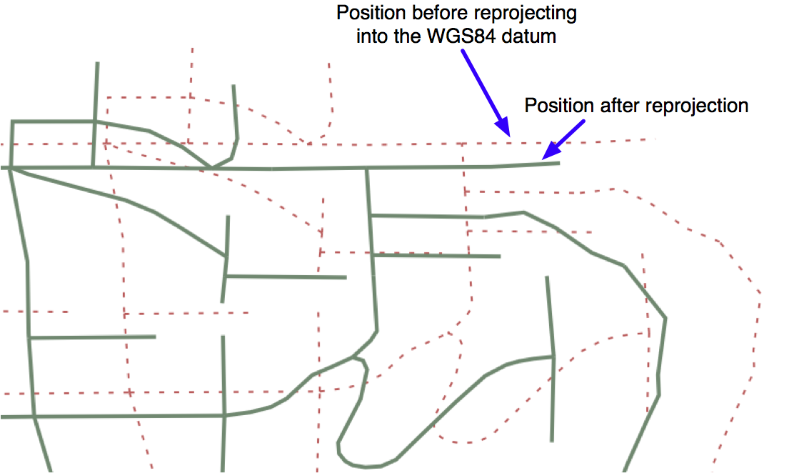
如果我们现在使用 WGS84 基准面绘制重投影后的特征,特征将出现在正确的位置:
For this example, we will need to obtain some geospatial data that uses the NAD27 datum. This datum dates back to 1927, and was commonly used for North American geospatial analysis up until the 1980s when it was replaced by NAD83.
ESRI makes available a set of TIGER/Line files from the 2000 US census, converted into shapefile format. These files can be downloaded from:
http://esri.com/data/download/census2000-tigerline/index.html
For the 2000 census data, the TIGER/Line files were all in NAD83, with the exception of Alaska which used the older NAD27 datum. So we can use the preceding site to download a shapefile containing features in NAD27. Go to the site, click on the Preview and Download hyperlink, and then choose Alaska from the drop-down menu. Select the Line Features - Roads layer, then click on the Submit Selection button.
This data is divided up into individual counties. Click on the checkbox beside Anchorage, then click on the Proceed to Download button to download the shapefile containing road details in Anchorage. The resulting shapefile will be named tgr02020lkA.shp, and will be in a directory called lkA02020.
As described on the website, this data uses the NAD27 datum. If we were to assume this shapefile used the WSG83 datum, all the features would be in the wrong place:
To make the features appear in the correct place, and to be able to combine these features with other data that uses the WGS84 datum, we need to convert the shapefile to use WGS84. Changing a shapefile from one datum to another requires the same basic process we used earlier to change a shapefile from one projection to another: first you choose the source and destination datums, and define a coordinate transformation to convert from one to the other:
srcDatum = osr.SpatialReference()
srcDatum.SetWellKnownGeogCS('NAD27')

dstDatum = osr.SpatialReference()
dstDatum.SetWellKnownGeogCS('WGS84')

transform = osr.CoordinateTransformation(srcDatum, dstDatum)
You then process each feature in the shapefile, transforming the feature’s geometry using the coordinate transformation:
for i in range(srcLayer.GetFeatureCount()):
    feature = srcLayer.GetFeature(i)
    geometry = feature.GetGeometryRef()
    geometry.Transform(transform)
Here is the complete Python program to convert the lkA02020 shapefile from the NAD27 datum to WGS84:
# changeDatum.py

import os, os.path, shutil
from osgeo import ogr
from osgeo import osr
from osgeo import gdal

# Define the source and destination datums, and a
# transformation object to convert from one to the other.

srcDatum = osr.SpatialReference()
srcDatum.SetWellKnownGeogCS('NAD27')

dstDatum = osr.SpatialReference()
dstDatum.SetWellKnownGeogCS('WGS84')

transform = osr.CoordinateTransformation(srcDatum, dstDatum)

# Open the source shapefile.

srcFile = ogr.Open("lkA02020/tgr02020lkA.shp")
srcLayer = srcFile.GetLayer(0)

# Create the dest shapefile, and give it the new projection.

if os.path.exists("lkA-reprojected"):
    shutil.rmtree("lkA-reprojected")
os.mkdir("lkA-reprojected")

driver = ogr.GetDriverByName("ESRI Shapefile")
dstPath = os.path.join("lkA-reprojected", "lkA02020.shp")
dstFile = driver.CreateDataSource(dstPath)
dstLayer = dstFile.CreateLayer("layer", dstDatum)

# Reproject each feature in turn.

for i in range(srcLayer.GetFeatureCount()):
    feature = srcLayer.GetFeature(i)
    geometry = feature.GetGeometryRef()
    newGeometry = geometry.Clone()
    newGeometry.Transform(transform)
    feature = ogr.Feature(dstLayer.GetLayerDefn())
    feature.SetGeometry(newGeometry)
    dstLayer.CreateFeature(feature)
    feature.Destroy()

# All done.

srcFile.Destroy()
dstFile.Destroy()
The preceding code assumes that the lkA02020 folder is in the same directory as the Python script itself. If you’ve placed this folder somewhere else, you’ll need to change the ogr.Open() statement to use the appropriate directory path.
If we now plot the reprojected features using the WGS84 datum, the features will appear in the correct place: