1.3 网络核心#
1.3 The Network Core
在我们已经了解了互联网的边缘之后,现在让我们深入探讨网络核心——由分组交换机和链路构成的网状结构,连接了互联网的各个终端系统。图 1.10 使用加粗阴影线高亮显示了网络核心部分。
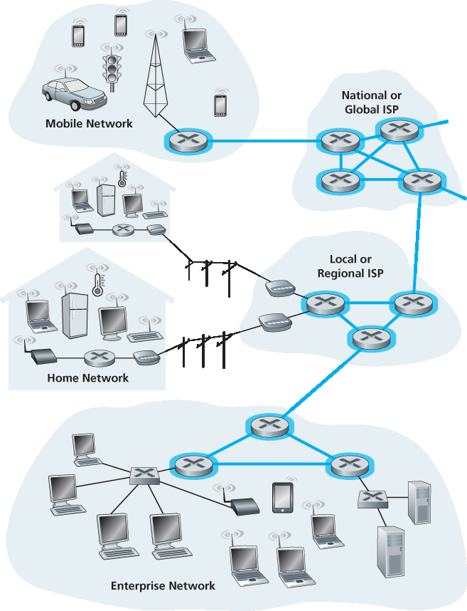
图 1.10 网络核心
Having examined the Internet’s edge, let us now delve more deeply inside the network core—the mesh of packet switches and links that interconnects the Internet’s end systems. Figure 1.10 highlights the network core with thick, shaded lines.
Figure 1.10 The network core
1.3.1 分组交换#
1.3.1 Packet Switching
在网络应用中,终端系统彼此交换 消息(messages)。消息可以包含应用设计者想要传输的任何内容。消息可以是控制信息(例如我们在 图 1.2 的握手例子中的 “Hi” 消息),也可以是数据,例如电子邮件、JPEG 图像或 MP3 音频文件。为了将消息从源终端系统发送到目的终端系统,源系统会将长消息分割为较小的数据块,称为 分组(packets)。在从源到目的的路径中,每个分组都通过通信链路和 分组交换机(packet switches) (主要包括 路由器(routers) 和 链路层交换机(link-layer switches))传输。每个通信链路上传输分组的速率等于该链路的 全部 传输速率。因此,如果一个源终端系统或分组交换机在速率为 R 位/秒的链路上传输一个 L 位的分组,则传输该分组所需时间为 L / R 秒。
In a network application, end systems exchange messages with each other. Messages can contain anything the application designer wants. Messages may perform a control function (for example, the “Hi” messages in our handshaking example in Figure 1.2 ) or can contain data, such as an e-mail message, a JPEG image, or an MP3 audio file. To send a message from a source end system to a destination end system, the source breaks long messages into smaller chunks of data known as packets. Between source and destination, each packet travels through communication links and packet switches (for which there are two predominant types, routers and link-layer switches). Packets are transmitted over each communication link at a rate equal to the full transmission rate of the link. So, if a source end system or a packet switch is sending a packet of L bits over a link with transmission rate R bits/sec, then the time to transmit the packet is L / R seconds.
存储-转发传输#
Store-and-Forward Transmission
大多数分组交换机在链路的输入端采用 存储-转发传输(store-and-forward transmission)。该方式要求交换机在开始传输分组的第一个比特之前,必须完整接收整个分组。为了更详细地了解这种机制,考虑一个简单网络,该网络由两个终端系统和一个中间路由器组成,如 图 1.11 所示。路由器通常连接多个链路,本例中只需将一个输入链路上的分组转发到唯一的输出链路上。源端系统有三个由 L 位组成的分组要发送。在图中的时间快照时,源已经传输了部分分组 1,分组 1 的前部已经到达路由器。由于采用存储-转发机制,路由器尚不能传输已接收的比特,而必须首先将其缓冲(即“存储”)。只有在完整接收整个分组后,路由器才能开始将其转发到输出链路。为了了解传输时延,我们现在来计算从源开始发送分组到目的端系统完全接收到该分组所需的总时间。(此处我们忽略传播时延,这将在 第 1.4 节 中讨论。)源在时间 0 开始发送,在 L/R 秒时,源完成发送,路由器也接收到整个分组;此后,路由器开始向目的系统发送该分组,并在 2L/R 秒时完成发送。因此,总时延为 2L/R。如果路由器在接收到部分比特后就立即转发,而不等待整个分组,则时延为 L/R。但如我们将在 第 1.4 节 中讨论的,路由器需要接收、存储并 处理 整个分组后才进行转发。
图 1.11 存储-转发分组交换
现在我们来计算从源开始发送第一个分组到目的端系统接收到所有三个分组所需的总时间。与前面一样,在 L/R 秒时,路由器开始转发第一个分组,同时源也开始发送第二个分组。到 2L/R 秒时,目的端系统收到第一个分组,路由器接收到第二个分组。以此类推,到 4L/R 秒时,目的端系统收到了全部三个分组。
现在考虑一般情况:一个分组从源到目的需经过 N 条传输速率为 R 的链路(中间有 N-1 个路由器)。根据上述逻辑,端到端时延为:
dend-to-end = N * L / R (1.1)
你现在可以尝试推导:在 N 条链路上传输 P 个分组的总时延为多少。
Most packet switches use store-and-forward transmission at the inputs to the links. Store-and-forward transmission means that the packet switch must receive the entire packet before it can begin to transmit the first bit of the packet onto the outbound link. To explore store-and-forward transmission in more detail, consider a simple network consisting of two end systems connected by a single router, as shown in Figure 1.11. A router will typically have many incident links, since its job is to switch an incoming packet onto an outgoing link; in this simple example, the router has the rather simple task of transferring a packet from one (input) link to the only other attached link. In this example, the source has three packets, each consisting of L bits, to send to the destination. At the snapshot of time shown in Figure 1.11, the source has transmitted some of packet 1, and the front of packet 1 has already arrived at the router. Because the router employs store-and-forwarding, at this instant of time, the router cannot transmit the bits it has received; instead it must first buffer (i.e., “store”) the packet’s bits. Only after the router has received all of the packet’s bits can it begin to transmit (i.e., “forward”) the packet onto the outbound link. To gain some insight into store-and-forward transmission, let’s now calculate the amount of time that elapses from when the source begins to send the packet until the destination has received the entire packet. (Here we will ignore propagation delay—the time it takes for the bits to travel across the wire at near the speed of light—which will be discussed in Section 1.4 .) The source begins to transmit at time 0; at time L/R seconds, the source has transmitted the entire packet, and the entire packet has been received and stored at the router (since there is no propagation delay). At time L/R seconds, since the router has just received the entire packet, it can begin to transmit the packet onto the outbound link towards the destination; at time 2L/R, the router has transmitted the entire packet, and the entire packet has been received by the destination. Thus, the total delay is 2L/R. If the switch instead forwarded bits as soon as they arrive (without first receiving the entire packet), then the total delay would be L/R since bits are not held up at the router. But, as we will discuss in Section 1.4, routers need to receive, store, and process the entire packet before forwarding.
Figure 1.11 Store-and-forward packet switching
Now let’s calculate the amount of time that elapses from when the source begins to send the first packet until the destination has received all three packets. As before, at time L/R, the router begins to forward the first packet. But also at time L/R the source will begin to send the second packet, since it has just finished sending the entire first packet. Thus, at time 2L/R, the destination has received the first packet and the router has received the second packet. Similarly, at time 3L/R, the destination has received the first two packets and the router has received the third packet. Finally, at time 4L/R the destination has received all three packets!
Let’s now consider the general case of sending one packet from source to destination over a path consisting of N links each of rate R (thus, there are N-1 routers between source and destination). Applying the same logic as above, we see that the end-to-end delay is:
dend-to-end=NLR (1.1)
You may now want to try to determine what the delay would be for P packets sent over a series of N links.
排队时延与分组丢失#
Queuing Delays and Packet Loss
每个分组交换机连接多个链路。对于每条链路,交换机都有一个 输出缓冲区(output buffer) (或称 输出队列 output queue),用于存储即将通过该链路发送的分组。输出缓冲在分组交换中发挥着关键作用。如果一个到达的分组要通过一条正忙于发送其他分组的链路,则该分组必须等待。这会引入输出缓冲的 排队时延(queuing delay)。该时延是变化的,取决于网络的拥塞程度。
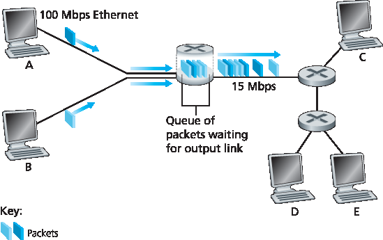
图 1.12 分组交换
由于缓冲空间是有限的,若缓冲已被其他分组占满,则新到的分组可能无法进入缓冲区。这种情况下就会发生 分组丢失(packet loss) —— 要么丢弃新到的分组,要么丢弃已排队的某个分组。
图 1.12 展示了一个简单的分组交换网络。与 图 1.11 一样,分组用三维“块”表示,其宽度表示分组的比特数。假设主机 A 和主机 B 都在向主机 E 发送分组,先通过 100 Mbps 的以太网链路发送到第一个路由器,然后由该路由器转发到 15 Mbps 链路上。如果某一时间段内,路由器收到的总速率(换算为 bit/s)超过了 15 Mbps,那么这些分组将在输出缓冲中排队等待,造成拥塞。例如,若 A 和 B 同时连续发送五个分组,大部分分组都需要在队列中等待。这种情况就如我们在现实生活中排队等候银行柜员或高速公路收费站一样。我们将在 第 1.4 节 中进一步探讨这种排队时延。
Each packet switch has multiple links attached to it. For each attached link, the packet switch has an output buffer (also called an output queue), which stores packets that the router is about to send into that link. The output buffers play a key role in packet switching. If an arriving packet needs to be transmitted onto a link but finds the link busy with the transmission of another packet, the arriving packet must wait in the output buffer. Thus, in addition to the store-and-forward delays, packets suffer output buffer queuing delays. These delays are variable and depend on the level of congestion in the network.
Figure 1.12 Packet switching
Since the amount of buffer space is finite, an arriving packet may find that the buffer is completely full with other packets waiting for transmission. In this case, packet loss will occur—either the arriving packet or one of the already-queued packets will be dropped.
Figure 1.12 illustrates a simple packet-switched network. As in Figure 1.11, packets are represented by three-dimensional slabs. The width of a slab represents the number of bits in the packet. In this figure, all packets have the same width and hence the same length. Suppose Hosts A and B are sending packets to Host E. Hosts A and B first send their packets along 100 Mbps Ethernet links to the first router. The router then directs these packets to the 15 Mbps link. If, during a short interval of time, the arrival rate of packets to the router (when converted to bits per second) exceeds 15 Mbps, congestion will occur at the router as packets queue in the link’s output buffer before being transmitted onto the link. For example, if Host A and B each send a burst of five packets back-to-back at the same time, then most of these packets will spend some time waiting in the queue. The situation is, in fact, entirely analogous to many common-day situations—for example, when we wait in line for a bank teller or wait in front of a tollbooth. We’ll examine this queuing delay in more detail in Section 1.4.
转发表与路由协议#
Forwarding Tables and Routing Protocols
前面我们提到,路由器将到达的分组从一个链路转发到另一个链路。但它是如何决定该分组应转发到哪条链路的呢?不同类型的计算机网络中,分组转发方式不同。下面简要介绍互联网中的做法。
在互联网中,每个终端系统都有一个称为 IP 地址的地址。当源系统要向目的系统发送分组时,会在分组的首部中写入目的 IP 地址。就像邮政地址一样,IP 地址具有层次结构。当分组到达某个路由器时,该路由器检查该地址的一部分,并将分组转发给相邻路由器。具体地说,每个路由器都有一个 转发表(forwarding table),用于将目标地址(或其一部分)映射到该路由器的输出链路。当分组到达时,路由器使用目的地址查表,决定应通过哪条链路转发。
这个过程类似于开车不看地图而一路问路。例如,Joe 从费城开车到佛罗里达奥兰多的 156 Lakeside Drive。他首先问加油站工作人员如何前往,该工作人员提取地址中的佛罗里达部分并告诉他进入 I-95 南段高速,然后在佛州再问路。Joe 在杰克逊维尔再次问路,得到前往 Daytona Beach 的指示;在 Daytona Beach 又问路,最后在奥兰多问到了具体街道和门牌号。这些“问路人”就像是路由器。
我们了解到,路由器通过目的地址查找转发表,确定转发链路。但转发表是如何配置的?是否需要人工逐一配置?互联网采用的是自动化方式,使用若干特殊的 路由协议(routing protocols) 来设置转发表。比如,某个协议可能计算从每个路由器到所有目的地的最短路径,并据此设置转发表。
你是否想亲自看看在互联网上分组的端到端路径?可以访问网站 www.traceroute.org,选择一个国家的源点,然后追踪到你电脑的路径。(有关 Traceroute 的详细内容见 第 1.4 节。)
Earlier, we said that a router takes a packet arriving on one of its attached communication links and forwards that packet onto another one of its attached communication links. But how does the router determine which link it should forward the packet onto? Packet forwarding is actually done in different ways in different types of computer networks. Here, we briefly describe how it is done in the Internet.
In the Internet, every end system has an address called an IP address. When a source end system wants to send a packet to a destination end system, the source includes the destination’s IP address in the packet’s header. As with postal addresses, this address has a hierarchical structure. When a packet arrives at a router in the network, the router examines a portion of the packet’s destination address and forwards the packet to an adjacent router. More specifically, each router has a forwarding table that maps destination addresses (or portions of the destination addresses) to that router’s outbound links. When a packet arrives at a router, the router examines the address and searches its forwarding table, using this destination address, to find the appropriate outbound link. The router then directs the packet to this outbound link.
The end-to-end routing process is analogous to a car driver who does not use maps but instead prefers to ask for directions. For example, suppose Joe is driving from Philadelphia to 156 Lakeside Drive in Orlando, Florida. Joe first drives to his neighborhood gas station and asks how to get to 156 Lakeside Drive in Orlando, Florida. The gas station attendant extracts the Florida portion of the address and tells Joe that he needs to get onto the interstate highway I-95 South, which has an entrance just next to the gas station. He also tells Joe that once he enters Florida, he should ask someone else there. Joe then takes I-95 South until he gets to Jacksonville, Florida, at which point he asks another gas station attendant for directions. The attendant extracts the Orlando portion of the address and tells Joe that he should continue on I-95 to Daytona Beach and then ask someone else. In Daytona Beach, another gas station attendant also extracts the Orlando portion of the address and tells Joe that he should take I-4 directly to Orlando. Joe takes I-4 and gets off at the Orlando exit. Joe goes to another gas station attendant, and this time the attendant extracts the Lakeside Drive portion of the address and tells Joe the road he must follow to get to Lakeside Drive. Once Joe reaches Lakeside Drive, he asks a kid on a bicycle how to get to his destination. The kid extracts the 156 portion of the address and points to the house. Joe finally reaches his ultimate destination. In the above analogy, the gas station attendants and kids on bicycles are analogous to routers.
We just learned that a router uses a packet’s destination address to index a forwarding table and determine the appropriate outbound link. But this statement begs yet another question: How do forwarding tables get set? Are they configured by hand in each and every router, or does the Internet use a more automated procedure? This issue will be studied in depth in Chapter 5. But to whet your appetite here, we’ll note now that the Internet has a number of special routing protocols that are used to automatically set the forwarding tables. A routing protocol may, for example, determine the shortest path from each router to each destination and use the shortest path results to configure the forwarding tables in the routers.
How would you actually like to see the end-to-end route that packets take in the Internet? We now invite you to get your hands dirty by interacting with the Trace-route program. Simply visit the site www.traceroute.org , choose a source in a particular country, and trace the route from that source to your computer. (For a discussion of Traceroute, see Section 1.4.)
1.3.2 电路交换#
1.3.2 Circuit Switching
在链路与交换机构成的网络中,传输数据有两种基本方式: 电路交换(circuit switching) 与 分组交换(packet switching)。前一小节已介绍了分组交换网络,本节我们转而关注电路交换网络。
在电路交换网络中,为了在通信会话期间为终端系统间的通信提供服务,路径上的所需资源(如缓冲区、链路传输速率)在会话期间会被 预留。而在分组交换网络中,这些资源 不会 被预留;通信会话的消息按需使用资源,因此可能不得不等待(即排队)以使用某条链路。一个简单的类比是两家餐厅,一家需要预订,另一家不接受也不需要预订。对于需要预订的餐厅,我们出门前必须先打电话确认,但到达餐厅后原则上可以立刻入座点餐。而不需要预订的餐厅虽然无需提前准备,但到了之后可能需要排队等待。
传统电话网络是电路交换网络的例子。设想某人想通过电话网络发送语音或传真给另一人。在发送之前,网络必须在发送方和接收方之间建立一条连接。这是一条真正的连接,路径上的交换机会为其维持连接状态。在电话术语中,这种连接称为 电路(circuit)。建立电路的同时,网络也会在路径上的链路中预留一段恒定传输速率(代表链路传输能力的一部分),用于整个会话期间的通信。因此,发送方可以以保证的恒定速率将数据传送至接收方。
图 1.13 展示了一个电路交换网络。图中,四个电路交换机通过四条链路互联。每条链路可以支持四条电路,因此每条链路最多支持四个同时连接。各主机(如 PC 或工作站)直接连接到某个交换机。当两个主机需要通信时,网络会在它们之间建立一条专用的 端到端连接。例如,主机 A 想与主机 B 通信,网络必须分别在两条链路中预留一条电路。在此例中,端到端连接分别使用第一条链路的第二条电路和第二条链路的第四条电路。因为每条链路支持四条电路,每个连接在通信期间可独占链路总带宽的四分之一。例如,如果相邻交换机之间的链路速率为 1 Mbps,则每条端到端的电路连接拥有 250 kbps 的专用带宽。
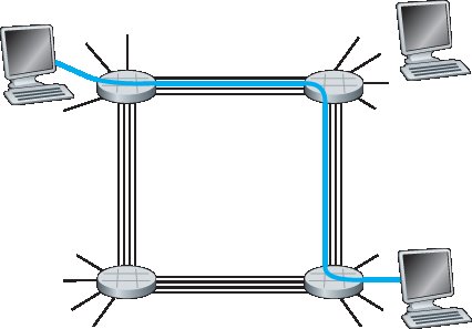
图 1.13 一个由四个交换机和四条链路构成的简单电路交换网络
相比之下,在分组交换网络(如互联网)中,若某主机想向另一主机发送分组,该分组同样会经过一系列通信链路传输。但与电路交换不同,分组无需预留任何链路资源。如果某条链路因同时有其他分组要传输而发生拥塞,则该分组将在发送侧链路缓冲中等待并产生延迟。互联网采取的是尽力而为的方式来及时传递分组,但并不提供任何保证。
There are two fundamental approaches to moving data through a network of links and switches: circuit switching and packet switching. Having covered packet-switched networks in the previous subsection, we now turn our attention to circuit-switched networks.
In circuit-switched networks, the resources needed along a path (buffers, link transmission rate) to provide for communication between the end systems are reserved for the duration of the communication session between the end systems. In packet-switched networks, these resources are not reserved; a session’s messages use the resources on demand and, as a consequence, may have to wait (that is, queue) for access to a communication link. As a simple analogy, consider two restaurants, one that requires reservations and another that neither requires reservations nor accepts them. For the restaurant that requires reservations, we have to go through the hassle of calling before we leave home. But when we arrive at the restaurant we can, in principle, immediately be seated and order our meal. For the restaurant that does not require reservations, we don’t need to bother to reserve a table. But when we arrive at the restaurant, we may have to wait for a table before we can be seated.
Traditional telephone networks are examples of circuit-switched networks. Consider what happens when one person wants to send information (voice or facsimile) to another over a telephone network. Before the sender can send the information, the network must establish a connection between the sender and the receiver. This is a bona fide connection for which the switches on the path between the sender and receiver maintain connection state for that connection. In the jargon of telephony, this connection is called a circuit. When the network establishes the circuit, it also reserves a constant transmission rate in the network’s links (representing a fraction of each link’s transmission capacity) for the duration of the connection. Since a given transmission rate has been reserved for this sender-to- receiver connection, the sender can transfer the data to the receiver at the guaranteed constant rate.
Figure 1.13 illustrates a circuit-switched network. In this network, the four circuit switches are interconnected by four links. Each of these links has four circuits, so that each link can support four simultaneous connections. The hosts (for example, PCs and workstations) are each directly connected to one of the switches. When two hosts want to communicate, the network establishes a dedicated end- to-end connection between the two hosts. Thus, in order for Host A to communicate with Host B, the network must first reserve one circuit on each of two links. In this example, the dedicated end-to-end connection uses the second circuit in the first link and the fourth circuit in the second link. Because each link has four circuits, for each link used by the end-to-end connection, the connection gets one fourth of the link’s total transmission capacity for the duration of the connection. Thus, for example, if each link between adjacent switches has a transmission rate of 1 Mbps, then each end-to-end circuit-switch connection gets 250 kbps of dedicated transmission rate.
Figure 1.13 A simple circuit-switched network consisting of four switches and four links
In contrast, consider what happens when one host wants to send a packet to another host over a packet-switched network, such as the Internet. As with circuit switching, the packet is transmitted over a series of communication links. But different from circuit switching, the packet is sent into the network without reserving any link resources whatsoever. If one of the links is congested because other packets need to be transmitted over the link at the same time, then the packet will have to wait in a buffer at the sending side of the transmission link and suffer a delay. The Internet makes its best effort to deliver packets in a timely manner, but it does not make any guarantees.
电路交换中的复用#
Multiplexing in Circuit-Switched Networks
链路中的电路通常采用 频分复用(FDM) 或 时分复用(TDM) 实现。FDM 将链路的频谱划分为多个频带,每条连接在整个会话期间占用一个频带。在电话网络中,通常每条连接占用 4 kHz(即 4000 Hz)带宽,这一带宽也称为 带宽(bandwidth)。FM 广播电台也使用 FDM,将 88 MHz 至 108 MHz 的频谱划分给不同电台。
TDM 则将时间划分为固定长度的帧,每帧再划分为固定数量的时隙。网络在建立连接后,会在每帧中为该连接分配一个专用时隙,该时隙仅供该连接使用。
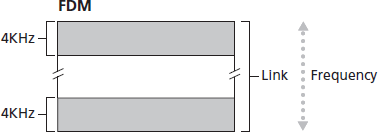
图 1.14 FDM 每条电路持续占据部分带宽,TDM 每条电路在短暂时隙内周期性占用全部带宽
图 1.14 展示了一条支持最多四条电路的链路的 FDM 与 TDM 示例。FDM 将频域分为四个带宽为 4 kHz 的频段。TDM 将时间划分为帧,每帧含有四个时隙;每条电路在每帧中占据同一专用时隙。TDM 中电路的传输速率等于帧率乘以每个时隙的比特数。例如,如果链路每秒传输 8000 帧,每个时隙 8 比特,则每条电路的速率为 64 kbps。
分组交换的支持者认为电路交换存在资源浪费问题,因为在 静默期(silent periods) 期间,专用电路处于空闲状态,其他连接无法使用其资源。例如,通话过程中一方沉默时,其占用的频段或时隙无法用于其他连接。再如放射科医生远程查看 X 光图像时,虽然连接已建立,但在观察图像期间网络资源处于未使用状态,从而造成浪费。此外,建立端到端电路并分配带宽也较复杂,需使用专门的信令协议协调路径上所有交换机的操作。
在结束电路交换讨论之前,我们来看一个数值例子。假设主机 A 要通过电路交换网络向主机 B 发送一个 640,000 位的文件。网络中所有链路使用 TDM,含 24 个时隙,位率为 1.536 Mbps。假设建立端到端电路需 500 毫秒。每条电路的传输速率为 1.536 Mbps / 24 = 64 kbps,因此发送文件需 640,000 / 64,000 = 10 秒。加上建立连接所需时间,总共约 10.5 秒。注意该传输时间与链路数无关:无论中间经过 1 条链路还是 100 条,传输时间仍为 10 秒。(实际端到端时延还包括传播时延,详见 第 1.4 节。)
A circuit in a link is implemented with either frequency-division multiplexing (FDM) or time-division multiplexing (TDM). With FDM, the frequency spectrum of a link is divided up among the connections established across the link. Specifically, the link dedicates a frequency band to each connection for the duration of the connection. In telephone networks, this frequency band typically has a width of 4 kHz (that is, 4,000 hertz or 4,000 cycles per second). The width of the band is called, not surprisingly, the bandwidth. FM radio stations also use FDM to share the frequency spectrum between 88 MHz and 108 MHz, with each station being allocated a specific frequency band.
For a TDM link, time is divided into frames of fixed duration, and each frame is divided into a fixed number of time slots. When the network establishes a connection across a link, the network dedicates one time slot in every frame to this connection. These slots are dedicated for the sole use of that connection, with one time slot available for use (in every frame) to transmit the connection’s data.
Figure 1.14 With FDM, each circuit continuously gets a fraction of the bandwidth. With TDM, each circuit gets all of the bandwidth periodically during brief intervals of time (that is, during slots)
Figure 1.14 illustrates FDM and TDM for a specific network link supporting up to four circuits. For FDM, the frequency domain is segmented into four bands, each of bandwidth 4 kHz. For TDM, the time domain is segmented into frames, with four time slots in each frame; each circuit is assigned the same dedicated slot in the revolving TDM frames. For TDM, the transmission rate of a circuit is equal to the frame rate multiplied by the number of bits in a slot. For example, if the link transmits 8,000 frames per second and each slot consists of 8 bits, then the transmission rate of each circuit is 64 kbps.
Proponents of packet switching have always argued that circuit switching is wasteful because the dedicated circuits are idle during silent periods. For example, when one person in a telephone call stops talking, the idle network resources (frequency bands or time slots in the links along the connection’s route) cannot be used by other ongoing connections. As another example of how these resources can be underutilized, consider a radiologist who uses a circuit-switched network to remotely access a series of x-rays. The radiologist sets up a connection, requests an image, contemplates the image, and then requests a new image. Network resources are allocated to the connection but are not used (i.e., are wasted) during the radiologist’s contemplation periods. Proponents of packet switching also enjoy pointing out that establishing end-to-end circuits and reserving end-to-end transmission capacity is complicated and requires complex signaling software to coordinate the operation of the switches along the end-to-end path.
Before we finish our discussion of circuit switching, let’s work through a numerical example that should shed further insight on the topic. Let us consider how long it takes to send a file of 640,000 bits from Host A to Host B over a circuit-switched network. Suppose that all links in the network use TDM with 24 slots and have a bit rate of 1.536 Mbps. Also suppose that it takes 500 msec to establish an end-to-end circuit before Host A can begin to transmit the file. How long does it take to send the file? Each circuit has a transmission rate of (1.536 Mbps)/24=64 kbps, so it takes (640,000 bits)/(64 kbps)=10 seconds to transmit the file. To this 10 seconds we add the circuit establishment time, giving 10.5 seconds to send the file. Note that the transmission time is independent of the number of links: The transmission time would be 10 seconds if the end-to-end circuit passed through one link or a hundred links. (The actual end-to-end delay also includes a propagation delay; see Section 1.4 .)
分组交换与电路交换对比#
Packet Switching Versus Circuit Switching
我们已分别介绍电路交换与分组交换,下面进行对比。分组交换的批评者认为其不适合实时服务(如电话或视频会议),因为其端到端时延是可变且不可预测的,主要由于排队时延不确定。而支持者则认为:(1)分组交换比电路交换更好地共享带宽;(2)其实现更简单、高效且成本更低。关于该对比的深入讨论可参见 [Molinero-Fernandez 2002]。一般而言,不喜欢预约餐厅的人更偏爱分组交换。
为什么分组交换更高效?来看一个简单例子。假设用户共享 1 Mbps 链路,每个用户在活动时以 100 kbps 速率产生数据,在非活动时不产生数据。设用户仅有 10% 时间处于活跃状态(其余时间喝咖啡)。在电路交换中,每个用户始终需预留 100 kbps,例如使用 TDM 时,若一秒划分为十个 100ms 时隙,则每用户占一个时隙,最多支持 10 (=1 Mbps / 100 kbps) 个用户。
而在分组交换中,用户活跃概率为 0.1。若有 35 个用户,超过 10 个用户同时活跃的概率约为 0.0004(详见 课后练习 P8)。在 10 个及以下用户同时活跃时,链路总输入速率不超过 1 Mbps,分组传输几乎无延迟,表现类似电路交换。当活跃用户超过 10 个时,输出队列开始增长,直至输入速率回落。由于高于 10 个用户同时活跃的概率极小,分组交换在维持相似性能的同时支持用户数量是电路交换的三倍以上。
再看第二个例子。假设有 10 个用户,其中一个用户突然发送 1000 个 1000 位的分组,其余用户保持静默。若采用 10 时隙的 TDM 电路交换,每帧中仅有一个时隙可用于该用户,其余时隙空闲。传输所有分组需 10 秒。而在分组交换中,该用户可独占 1 Mbps 链路速率,在 1 秒内传完全部数据。
上述例子说明:在多数据流共享链路带宽时,分组交换的性能可优于电路交换。电路交换预先分配带宽,不管是否真正使用,未用部分被浪费;分组交换按需分配,仅在有分组需传输时才占用带宽。
虽然今天的通信网络中两者并存,但总体趋势偏向分组交换。甚至许多传统电路交换电话网络也逐渐向分组交换演进,尤其是在昂贵的国际段落中,通常采用分组交换方式。
Having described circuit switching and packet switching, let us compare the two. Critics of packet switching have often argued that packet switching is not suitable for real-time services (for example, telephone calls and video conference calls) because of its variable and unpredictable end-to-end delays (due primarily to variable and unpredictable queuing delays). Proponents of packet switching argue that (1) it offers better sharing of transmission capacity than circuit switching and (2) it is simpler, more efficient, and less costly to implement than circuit switching. An interesting discussion of packet switching versus circuit switching is [Molinero-Fernandez 2002]. Generally speaking, people who do not like to hassle with restaurant reservations prefer packet switching to circuit switching.
Why is packet switching more efficient? Let’s look at a simple example. Suppose users share a 1 Mbps link. Also suppose that each user alternates between periods of activity, when a user generates data at a constant rate of 100 kbps, and periods of inactivity, when a user generates no data. Suppose further that a user is active only 10 percent of the time (and is idly drinking coffee during the remaining 90 percent of the time). With circuit switching, 100 kbps must be reserved for each user at all times. For example, with circuit-switched TDM, if a one-second frame is divided into 10 time slots of 100 ms each, then each user would be allocated one time slot per frame.
Thus, the circuit-switched link can support only 10(=1 Mbps/100 kbps) simultaneous users. With packet switching, the probability that a specific user is active is 0.1 (that is, 10 percent). If there are 35 users, the probability that there are 11 or more simultaneously active users is approximately 0.0004. (Homework Problem P8 outlines how this probability is obtained.) When there are 10 or fewer simultaneously active users (which happens with probability 0.9996), the aggregate arrival rate of data is less than or equal to 1 Mbps, the output rate of the link. Thus, when there are 10 or fewer active users, users’ packets flow through the link essentially without delay, as is the case with circuit switching. When there are more than 10 simultaneously active users, then the aggregate arrival rate of packets exceeds the output capacity of the link, and the output queue will begin to grow. (It continues to grow until the aggregate input rate falls back below 1 Mbps, at which point the queue will begin to diminish in length.) Because the probability of having more than 10 simultaneously active users is minuscule in this example, packet switching provides essentially the same performance as circuit switching, but does so while allowing for more than three times the number of users.
Let’s now consider a second simple example. Suppose there are 10 users and that one user suddenly generates one thousand 1,000-bit packets, while other users remain quiescent and do not generate packets. Under TDM circuit switching with 10 slots per frame and each slot consisting of 1,000 bits, the active user can only use its one time slot per frame to transmit data, while the remaining nine time slots in each frame remain idle. It will be 10 seconds before all of the active user’s one million bits of data has been transmitted. In the case of packet switching, the active user can continuously send its packets at the full link rate of 1 Mbps, since there are no other users generating packets that need to be multiplexed with the active user’s packets. In this case, all of the active user’s data will be transmitted within 1 second.
The above examples illustrate two ways in which the performance of packet switching can be superior to that of circuit switching. They also highlight the crucial difference between the two forms of sharing a link’s transmission rate among multiple data streams. Circuit switching pre-allocates use of the transmission link regardless of demand, with allocated but unneeded link time going unused. Packet switching on the other hand allocates link use on demand. Link transmission capacity will be shared on a packet-by-packet basis only among those users who have packets that need to be transmitted over the link.
Although packet switching and circuit switching are both prevalent in today’s telecommunication networks, the trend has certainly been in the direction of packet switching. Even many of today’s circuit- switched telephone networks are slowly migrating toward packet switching. In particular, telephone networks often use packet switching for the expensive overseas portion of a telephone call.
1.3.3 网络的网络#
1.3.3 A Network of Networks
我们前面看到,端系统(如个人电脑、智能手机、Web 服务器、邮件服务器等)是通过接入 ISP 连接到互联网的。接入 ISP 可以通过多种接入技术(包括 DSL、有线电视、FTTH、Wi-Fi 和蜂窝网络)提供有线或无线连接。需要注意的是,接入 ISP 不一定是电信或有线电视公司;它也可以是大学(为学生、教职员工提供互联网接入),或者公司(为员工提供接入)。
但仅仅将终端用户和内容提供者连接到接入 ISP,并不能解决让数十亿终端系统互联的整个难题。要完成这块拼图,还必须让这些接入 ISP 相互连接。要做到这一点,需要构建一个 网络的网络(network of networks)。理解这一术语,是理解互联网的关键。
随着时间推移,构成互联网的网络体系结构逐步演化为一个极为复杂的结构。这种演化在很大程度上由经济和国家政策推动,而非完全出于性能考虑。为了理解今天的互联网结构,我们将逐步构建一系列网络结构,每一种都更接近当今复杂的互联网。请记住总体目标:连接所有接入 ISP,以便所有终端系统能够互相发送分组。
一种天真的做法是让每个接入 ISP 与所有其他接入 ISP 直接连接。但这种全互联网状结构对接入 ISP 来说成本过高,因为这要求它们分别与世界上数十万个其他接入 ISP 建立通信链路。
我们提出的第一个结构,称为 网络结构 1(Network Structure 1),将所有接入 ISP 连接到一个 全球传输 ISP(global transit ISP)。这个假想的全球传输 ISP 是由遍布全球的路由器和通信链路构成的网络,且在每个接入 ISP 附近至少部署一个路由器。当然,构建如此庞大的网络代价昂贵。为了盈利,该全球 ISP 会向每个接入 ISP 收取连接费用,费用与该 ISP 与全球 ISP 的流量量相关(但不一定成正比)。由于接入 ISP 向全球传输 ISP 支付费用,因此称接入 ISP 为 客户(customer),而全球传输 ISP 为 提供者(provider)。
如果某公司构建并运营了一个盈利的全球传输 ISP,其他公司自然也会竞争,构建自己的全球传输 ISP。这就形成了 网络结构 2(Network Structure 2),由数十万个接入 ISP 和 多个 全球传输 ISP 组成。接入 ISP 更倾向于网络结构 2,因为它们可以根据价格和服务在多个全球传输 ISP 之间做出选择。但要注意,全球传输 ISP 之间也必须互联:否则连接到不同全球传输 ISP 的接入 ISP 无法通信。
刚描述的网络结构 2 是一个两层层级结构,顶层为全球传输 ISP,底层为接入 ISP。这种结构假定全球传输 ISP 能且愿意接近每一个接入 ISP。但现实中,即便有些 ISP 在全球范围内覆盖广泛,并直接连接很多接入 ISP,也没有任何 ISP 能在全球所有城市部署节点。相反,在每个地区可能存在一个 区域 ISP(regional ISP),负责连接该地区的接入 ISP。每个区域 ISP 再连接到 一级 ISP(tier-1 ISP)。一级 ISP 类似于我们假想的全球传输 ISP;但一级 ISP 实际存在,它们不一定覆盖全球每个城市。一级 ISP 的数量约为十几个,包括 Level 3、AT&T、Sprint 和 NTT。有趣的是,没有组织对一级 ISP 身份进行正式认证——俗话说,如果你需要问自己是不是圈内人,那你多半不是。
回到网络的网络结构,不仅存在多个竞争的一级 ISP,在同一地区也可能存在多个区域 ISP。在这种层级结构中,每个接入 ISP 向其连接的区域 ISP 付费,每个区域 ISP 向其连接的一级 ISP 付费。(接入 ISP 也可以直接连接到一级 ISP,此时向其付费。)因此在每一层级都存在客户-提供者关系。注意,一级 ISP 位于层级顶端,不向任何其他 ISP 付费。
此外,有些地区可能还有更大范围的区域 ISP(例如覆盖整个国家),供较小的区域 ISP 连接,然后再连接到一级 ISP。例如在中国,各城市的接入 ISP 连接到省级 ISP,省级 ISP 再连接到国家级 ISP,最终连接到一级 ISP [Tian 2012]。我们将这种多层级但仍较粗略的互联网结构称为 网络结构 3(Network Structure 3)。
若要构建一个更贴近当今互联网的网络,我们需要在网络结构 3 基础上加入接入点(PoP)、多宿(multi-homing)、对等(peering)以及互联网交换点(IXP)。PoP 存在于除接入 ISP 以外的所有层级。PoP(point of presence) 是指服务提供者网络中一组位于同一地点的路由器,客户 ISP 可连接至此处。客户网络要连接某个提供者的 PoP,可以从第三方电信运营商租用高速链路,将其路由器直接接入 PoP 的路由器。
除一级 ISP 外的 ISP 均可选择 多宿(multi-home),即连接两个或多个上游 ISP。例如接入 ISP 可连接两个区域 ISP,或连接两个区域 ISP 再加一个一级 ISP;同样,区域 ISP 可连接多个一级 ISP。当 ISP 采用多宿方式时,即便某个提供者故障,也可继续通过其他连接接入互联网。
如前所述,客户 ISP 需向提供者 ISP 支付费用以获得全球互联能力,金额与其交换的流量相关。为了降低成本,位于同一层级、地理位置接近的两个 ISP 可选择 对等(peering),即直接连接各自网络,使它们之间的流量不再通过上游中转。通常,两家对等的 ISP 之间是 无结算(settlement-free) 的,即互不收费。如前所述,一级 ISP 之间也是无结算对等。关于对等与客户-提供者关系的通俗讨论,参见 [Van der Berg 2008]。
基于同样考虑,第三方公司还可以建立 互联网交换点(IXP),即多个 ISP 实现对等的集中接入点。IXP 通常位于独立建筑中,内部配备交换设备 [Ager 2012]。截至目前,全球已有超过 400 个 IXP [IXP List 2016]。我们将包括接入 ISP、区域 ISP、一级 ISP、PoP、多宿、对等、IXP 在内的这一生态称为 网络结构 4(Network Structure 4)。
最终我们到达 网络结构 5(Network Structure 5),即当今互联网。如 图 1.15 所示,网络结构 5 在结构 4 基础上新增了 内容提供商网络(content-provider networks)。Google 是这类网络的代表。截至目前,据估计 Google 在北美、欧洲、亚洲、南美和澳洲部署了 50 至 100 个数据中心。其中一些大型数据中心包含超过十万台服务器,小型数据中心也有数百台。Google 所有数据中心通过其私有 TCP/IP 网络互联,该网络虽然覆盖全球,但与公共互联网分离。重要的是,该私有网络仅承载与 Google 服务器有关的流量。
如 图 1.15 所示,Google 私有网络尝试通过与下层 ISP 建立对等(免费)连接,来 绕过 互联网的上层结构,这些连接可为直接连接,或通过 IXP 完成 [Labovitz 2010]。但由于很多接入 ISP 仍需通过一级 ISP 才能访问,Google 网络也会连接一级 ISP,并为此支付流量费用。通过建设自有网络,内容提供商不仅能减少向上层 ISP 支付的费用,还能更好地控制其服务最终如何传递到用户手中。Google 网络结构详见 第 2.6 节。
总之,当今互联网——一个“网络的网络”——结构复杂,包括十余个一级 ISP 和数十万个下层 ISP。这些 ISP 在覆盖范围上差异显著,有的跨洲跨洋,有的仅限于本地区域。下层 ISP 连接上层 ISP,上层 ISP 彼此互联。用户与内容提供商是下层 ISP 的客户,下层 ISP 是上层 ISP 的客户。近年来,主要内容提供商也开始建设自有网络,并尽可能直接连接至下层 ISP。
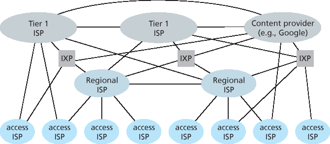
图 1.15 ISP 间互联结构
We saw earlier that end systems (PCs, smartphones, Web servers, mail servers, and so on) connect into the Internet via an access ISP. The access ISP can provide either wired or wireless connectivity, using an array of access technologies including DSL, cable, FTTH, Wi-Fi, and cellular. Note that the access ISP does not have to be a telco or a cable company; instead it can be, for example, a university (providing Internet access to students, staff, and faculty), or a company (providing access for its employees). But connecting end users and content providers into an access ISP is only a small piece of solving the puzzle of connecting the billions of end systems that make up the Internet. To complete this puzzle, the access ISPs themselves must be interconnected. This is done by creating a network of networks—understanding this phrase is the key to understanding the Internet.
Over the years, the network of networks that forms the Internet has evolved into a very complex structure. Much of this evolution is driven by economics and national policy, rather than by performance considerations. In order to understand today’s Internet network structure, let’s incrementally build a series of network structures, with each new structure being a better approximation of the complex Internet that we have today. Recall that the overarching goal is to interconnect the access ISPs so that all end systems can send packets to each other. One naive approach would be to have each access ISP directly connect with every other access ISP. Such a mesh design is, of course, much too costly for the access ISPs, as it would require each access ISP to have a separate communication link to each of the hundreds of thousands of other access ISPs all over the world.
Our first network structure, Network Structure 1, interconnects all of the access ISPs with a single global transit ISP. Our (imaginary) global transit ISP is a network of routers and communication links that not only spans the globe, but also has at least one router near each of the hundreds of thousands of access ISPs. Of course, it would be very costly for the global ISP to build such an extensive network. To be profitable, it would naturally charge each of the access ISPs for connectivity, with the pricing reflecting (but not necessarily directly proportional to) the amount of traffic an access ISP exchanges with the global ISP. Since the access ISP pays the global transit ISP, the access ISP is said to be a customer and the global transit ISP is said to be a provider.
Now if some company builds and operates a global transit ISP that is profitable, then it is natural for other companies to build their own global transit ISPs and compete with the original global transit ISP. This leads to Network Structure 2, which consists of the hundreds of thousands of access ISPs and multiple global transit ISPs. The access ISPs certainly prefer Network Structure 2 over Network Structure 1 since they can now choose among the competing global transit providers as a function of their pricing and services. Note, however, that the global transit ISPs themselves must interconnect: Otherwise access ISPs connected to one of the global transit providers would not be able to communicate with access ISPs connected to the other global transit providers.
Network Structure 2, just described, is a two-tier hierarchy with global transit providers residing at the top tier and access ISPs at the bottom tier. This assumes that global transit ISPs are not only capable of getting close to each and every access ISP, but also find it economically desirable to do so. In reality, although some ISPs do have impressive global coverage and do directly connect with many access ISPs, no ISP has presence in each and every city in the world. Instead, in any given region, there may be a regional ISP to which the access ISPs in the region connect. Each regional ISP then connects to tier-1 ISPs. Tier-1 ISPs are similar to our (imaginary) global transit ISP; but tier-1 ISPs, which actually do exist, do not have a presence in every city in the world. There are approximately a dozen tier-1 ISPs, including Level 3 Communications, AT&T, Sprint, and NTT. Interestingly, no group officially sanctions tier-1 status; as the saying goes—if you have to ask if you’re a member of a group, you’re probably not.
Returning to this network of networks, not only are there multiple competing tier-1 ISPs, there may be multiple competing regional ISPs in a region. In such a hierarchy, each access ISP pays the regional ISP to which it connects, and each regional ISP pays the tier-1 ISP to which it connects. (An access ISP can also connect directly to a tier-1 ISP, in which case it pays the tier-1 ISP). Thus, there is customer- provider relationship at each level of the hierarchy. Note that the tier-1 ISPs do not pay anyone as they are at the top of the hierarchy. To further complicate matters, in some regions, there may be a larger regional ISP (possibly spanning an entire country) to which the smaller regional ISPs in that region connect; the larger regional ISP then connects to a tier-1 ISP. For example, in China, there are access ISPs in each city, which connect to provincial ISPs, which in turn connect to national ISPs, which finally connect to tier-1 ISPs [Tian 2012]. We refer to this multi-tier hierarchy, which is still only a crude approximation of today’s Internet, as Network Structure 3.
To build a network that more closely resembles today’s Internet, we must add points of presence (PoPs), multi-homing, peering, and Internet exchange points (IXPs) to the hierarchical Network Structure 3. PoPs exist in all levels of the hierarchy, except for the bottom (access ISP) level. A PoP is simply a group of one or more routers (at the same location) in the provider’s network where customer ISPs can connect into the provider ISP. For a customer network to connect to a provider’s PoP, it can lease a high-speed link from a third-party telecommunications provider to directly connect one of its routers to a router at the PoP. Any ISP (except for tier-1 ISPs) may choose to multi-home, that is, to connect to two or more provider ISPs. So, for example, an access ISP may multi-home with two regional ISPs, or it may multi-home with two regional ISPs and also with a tier-1 ISP. Similarly, a regional ISP may multi-home with multiple tier-1 ISPs. When an ISP multi-homes, it can continue to send and receive packets into the Internet even if one of its providers has a failure.
As we just learned, customer ISPs pay their provider ISPs to obtain global Internet interconnectivity. The amount that a customer ISP pays a provider ISP reflects the amount of traffic it exchanges with the provider. To reduce these costs, a pair of nearby ISPs at the same level of the hierarchy can peer, that is, they can directly connect their networks together so that all the traffic between them passes over the direct connection rather than through upstream intermediaries. When two ISPs peer, it is typically settlement-free, that is, neither ISP pays the other. As noted earlier, tier-1 ISPs also peer with one another, settlement-free. For a readable discussion of peering and customer-provider relationships, see [Van der Berg 2008]. Along these same lines, a third-party company can create an Internet Exchange Point (IXP), which is a meeting point where multiple ISPs can peer together. An IXP is typically in a stand-alone building with its own switches [Ager 2012]. There are over 400 IXPs in the Internet today [IXP List 2016]. We refer to this ecosystem—consisting of access ISPs, regional ISPs, tier-1 ISPs, PoPs, multi-homing, peering, and IXPs—as Network Structure 4.
We now finally arrive at Network Structure 5, which describes today’s Internet. Network Structure 5, illustrated in Figure 1.15, builds on top of Network Structure 4 by adding content-provider networks. Google is currently one of the leading examples of such a content-provider network. As of this writing, it is estimated that Google has 50–100 data centers distributed across North America, Europe, Asia, South America, and Australia. Some of these data centers house over one hundred thousand servers, while other data centers are smaller, housing only hundreds of servers. The Google data centers are all interconnected via Google’s private TCP/IP network, which spans the entire globe but is nevertheless separate from the public Internet. Importantly, the Google private network only carries traffic to/from Google servers. As shown in Figure 1.15, the Google private network attempts to “bypass” the upper tiers of the Internet by peering (settlement free) with lower-tier ISPs, either by directly connecting with them or by connecting with them at IXPs [Labovitz 2010]. However, because many access ISPs can still only be reached by transiting through tier-1 networks, the Google network also connects to tier-1 ISPs, and pays those ISPs for the traffic it exchanges with them. By creating its own network, a content provider not only reduces its payments to upper-tier ISPs, but also has greater control of how its services are ultimately delivered to end users. Google’s network infrastructure is described in greater detail in Section 2.6.
In summary, today’s Internet—a network of networks—is complex, consisting of a dozen or so tier-1 ISPs and hundreds of thousands of lower-tier ISPs. The ISPs are diverse in their coverage, with some spanning multiple continents and oceans, and others limited to narrow geographic regions. The lower- tier ISPs connect to the higher-tier ISPs, and the higher-tier ISPs interconnect with one another. Users and content providers are customers of lower-tier ISPs, and lower-tier ISPs are customers of higher-tier ISPs. In recent years, major content providers have also created their own networks and connect directly into lower-tier ISPs where possible.
Figure 1.15 Interconnection of ISPs