4.2 路由器的内部结构#
4.2 What’s Inside a Router?
在我们概述了网络层中的数据平面与控制平面、转发与路由之间的重要区别,以及网络层的服务和功能之后,现在我们将注意力转向其转发功能——即将分组从路由器的输入链路实际转移到该路由器的适当输出链路。
图 4.4 展示了一个通用路由器架构的高级视图。可以识别出四个路由器组件:
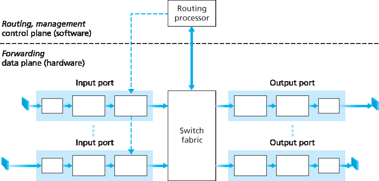
图 4.4 路由器架构
输入端口。一个 输入端口 执行多个关键功能。它执行物理层功能以终止到达路由器的物理链路;这体现在 图 4.4 中输入端口最左侧的盒子与输出端口最右侧的盒子。输入端口还执行链路层功能,以与入链路另一端的链路层互操作;这体现在输入端口与输出端口中间的盒子中。也许最关键的是,输入端口还执行查找功能;这将在输入端口最右侧的盒子中进行。此处会查阅转发表,以确定通过交换结构将到达分组转发至哪个路由器输出端口。控制分组(例如,承载路由协议信息的分组)会从输入端口转发至路由处理器。请注意,这里“端口”一词——指的是路由器的物理输入与输出接口——与 第 2 章 和 第 3 章 中讨论的网络应用和套接字相关的软件端口完全不同。实际上,路由器所支持的端口数可以从企业路由器中的少量端口,到 ISP 边缘路由器中支持数百个 10 Gbps 端口不等,因为入链路数量通常最多。例如,Juniper MX2020 边缘路由器支持最多 960 个 10 Gbps 以太网端口,整体系统容量为 80 Tbps [Juniper MX 2020 2016]。
交换结构。交换结构连接路由器的输入端口和输出端口。这个交换结构完全包含在路由器内部——是路由器内部的一个网络!
输出端口。一个 输出端口 存储来自交换结构的分组,并通过执行所需的链路层和物理层功能,将这些分组发送到出链路上。当链路是双向的(即双向传输流量)时,输出端口通常会与同一线路卡上的入链路输入端口配对。
路由处理器。路由处理器执行控制平面功能。在传统路由器中,它运行路由协议(我们将在 第 5.3 节 和 第 5.4 节 中学习),维护路由表和附属链路状态信息,并为路由器计算转发表。在 SDN 路由器中,路由处理器负责与远程控制器通信,以(除其他任务外)接收由远程控制器计算的转发表项,并将这些条目安装到路由器的输入端口中。路由处理器还执行我们将在 第 5.7 节 中学习的网络管理功能。
如 图 4.4 所示,路由器的输入端口、输出端口和交换结构几乎总是通过硬件实现的。为了理解为何需要硬件实现,考虑如下场景:若输入链路为 10 Gbps,而 IP 数据报为 64 字节,则输入端口只有 51.2 纳秒的时间来处理该数据报,然后可能就会有另一个数据报到达。如果在一张线路卡上组合了 N 个端口(实际中经常如此),则数据报处理流水线必须以 N 倍速率运行——对于软件实现而言,速度过快。转发硬件可以使用路由器厂商自己的硬件设计来实现,或者使用购买的商用芯片(例如由 Intel 和 Broadcom 等公司销售的芯片)构建。
虽然数据平面在纳秒级时间尺度上运行,但路由器的控制功能——执行路由协议、响应上升或下降的连接链路、与远程控制器通信(在 SDN 情况下)以及执行管理功能——是在毫秒或秒级时间尺度上运行的。这些 控制平面 功能通常通过软件实现,并在路由处理器(通常是传统 CPU)上执行。
在深入探讨路由器内部结构之前,让我们回顾本章开头的类比,其中分组转发被比作汽车进出交汇点。假设交汇点是一个环形交叉口,当一辆车驶入时,需要做一些处理。让我们思考完成这些处理所需的信息:
基于目的地的转发。假设汽车在入口站停下,并告知其最终目的地(不是本地环形交叉口,而是其旅程的最终目标)。入口站的一位服务员查阅目的地,确定通往该目的地的环形出口,并告知司机应驶出哪个出口。
通用转发。服务员也可以基于目的地之外的许多其他因素决定汽车应驶出的出口。例如,所选的出口可能依赖于汽车的来源地,例如车辆牌照所属的州。来自某些州的车辆可能被引导走一条通向目的地但道路较慢的出口,而来自其他州的车辆则可能被引导至通往目的地的高速公路。该决策还可能基于汽车的品牌、型号与年份。又或者,一辆不被认为适合上路的汽车可能会被禁止通过环形交叉口。在通用转发中,多种因素都可能影响服务员对某辆车所选出口的决定。
一旦汽车进入环形交叉口(其中可能充满了来自其他入口道路、驶向其他出口的车辆),它最终会从预定的出口驶离,并可能在该出口遇到其他同时离开的车辆。
我们可以很容易地在这个类比中识别出 图 4.4 中主要的路由器组件——入口道路和入口站对应于输入端口(带有查找功能,用于确定本地输出端口);环形交叉口对应于交换结构;环形出口道路对应于输出端口。基于这个类比,思考瓶颈可能出现的位置是有启发性的。如果车辆高速到达(例如该环形交叉口位于德国或意大利!),而服务员动作缓慢,会发生什么?服务员必须多快才能保证入口道路上不会堵车?即便服务员极快,如果车辆在环形交叉口内缓慢移动——是否仍可能堵车?如果几乎所有进入该环形交叉口的车辆都希望从同一个出口驶离,会不会在出口或其他位置形成堵塞?如果我们希望给不同车辆分配优先级,或阻止某些车辆进入环形交叉口,该如何操作?这些问题都类似于路由器与交换机设计人员必须面对的重要问题。
在接下来的小节中,我们将更详细地研究路由器的功能。[Iyer 2008,Chao 2001; Chuang 2005;Turner 1988;McKeown 1997a;Partridge 1998;Sopranos 2011] 对特定的路由器架构进行了讨论。为了简洁明了,在本节的开始部分,我们将假设转发决策仅基于分组的目的地址,而不是一组通用的分组首部字段。我们将在 第 4.4 节 中介绍更通用的分组转发情况。
Now that we’ve overviewed the data and control planes within the network layer, the important distinction between forwarding and routing, and the services and functions of the network layer, let’s turn our attention to its forwarding function—the actual transfer of packets from a router’s incoming links to the appropriate outgoing links at that router.
A high-level view of a generic router architecture is shown in Figure 4.4. Four router components can be identified:
Figure 4.4 Router architecture
Input ports. An input port performs several key functions. It performs the physical layer function of terminating an incoming physical link at a router; this is shown in the leftmost box of an input port and the rightmost box of an output port in Figure 4.4. An input port also performs link-layer functions needed to interoperate with the link layer at the other side of the incoming link; this is represented by the middle boxes in the input and output ports. Perhaps most crucially, a lookup function is also performed at the input port; this will occur in the rightmost box of the input port. It is here that the forwarding table is consulted to determine the router output port to which an arriving packet will be forwarded via the switching fabric. Control packets (for example, packets carrying routing protocol information) are forwarded from an input port to the routing processor. Note that the term “port” here —referring to the physical input and output router interfaces—is distinctly different from the softwareports associated with network applications and sockets discussed in Chapters 2 and 3. In practice, the number of ports supported by a router can range from a relatively small number in enterprise routers, to hundreds of 10 Gbps ports in a router at an ISP’s edge, where the number of incoming lines tends to be the greatest. The Juniper MX2020, edge router, for example, supports up to 960 10 Gbps Ethernet ports, with an overall router system capacity of 80 Tbps [Juniper MX 2020 2016].
Switching fabric. The switching fabric connects the router’s input ports to its output ports. This switching fabric is completely contained within the router—a network inside of a network router!
Output ports. An output port stores packets received from the switching fabric and transmits these packets on the outgoing link by performing the necessary link-layer and physical-layer functions. When a link is bidirectional (that is, carries traffic in both directions), an output port will typically be paired with the input port for that link on the same line card.
Routing processor. The routing processor performs control-plane functions. In traditional routers, it executes the routing protocols (which we’ll study in Sections 5.3 and 5.4), maintains routing tables and attached link state information, and computes the forwarding table for the router. In SDN routers, the routing processor is responsible for communicating with the remote controller in order to (among other activities) receive forwarding table entries computed by the remote controller, and install these entries in the router’s input ports. The routing processor also performs the network management functions that we’ll study in Section 5.7.
A router’s input ports, output ports, and switching fabric are almost always implemented in hardware, as shown in Figure 4.4. To appreciate why a hardware implementation is needed, consider that with a 10 Gbps input link and a 64-byte IP datagram, the input port has only 51.2 ns to process the datagram before another datagram may arrive. If N ports are combined on a line card (as is often done in practice), the datagram-processing pipeline must operate N times faster—far too fast for software implementation. Forwarding hardware can be implemented either using a router vendor’s own hardware designs, or constructed using purchased merchant-silicon chips (e.g., as sold by companies such as Intel and Broadcom).
While the data plane operates at the nanosecond time scale, a router’s control functions—executing the routing protocols, responding to attached links that go up or down, communicating with the remote controller (in the SDN case) and performing management functions—operate at the millisecond or second timescale. These control plane functions are thus usually implemented in software and execute on the routing processor (typically a traditional CPU).
Before delving into the details of router internals, let’s return to our analogy from the beginning of this chapter, where packet forwarding was compared to cars entering and leaving an interchange. Let’s suppose that the interchange is a roundabout, and that as a car enters the roundabout, a bit of processing is required. Let’s consider what information is required for this processing:
Destination-based forwarding. Suppose the car stops at an entry station and indicates its finaldestination (not at the local roundabout, but the ultimate destination of its journey). An attendant at the entry station looks up the final destination, determines the roundabout exit that leads to that final destination, and tells the driver which roundabout exit to take.
Generalized forwarding. The attendant could also determine the car’s exit ramp on the basis of many other factors besides the destination. For example, the selected exit ramp might depend on the car’s origin, for example the state that issued the car’s license plate. Cars from a certain set of states might be directed to use one exit ramp (that leads to the destination via a slow road), while cars from other states might be directed to use a different exit ramp (that leads to the destination via superhighway). The same decision might be made based on the model, make and year of the car. Or a car not deemed roadworthy might be blocked and not be allowed to pass through the roundabout. In the case of generalized forwarding, any number of factors may contribute to the attendant’s choice of the exit ramp for a given car.
Once the car enters the roundabout (which may be filled with other cars entering from other input roads and heading to other roundabout exits), it eventually leaves at the prescribed roundabout exit ramp, where it may encounter other cars leaving the roundabout at that exit.
We can easily recognize the principal router components in Figure 4.4 in this analogy—the entry road and entry station correspond to the input port (with a lookup function to determine to local outgoing port); the roundabout corresponds to the switch fabric; and the roundabout exit road corresponds to the output port. With this analogy, it’s instructive to consider where bottlenecks might occur. What happens if cars arrive blazingly fast (for example, the roundabout is in Germany or Italy!) but the station attendant is slow? How fast must the attendant work to ensure there’s no backup on an entry road? Even with a blazingly fast attendant, what happens if cars traverse the roundabout slowly—can backups still occur? And what happens if most of the cars entering at all of the roundabout’s entrance ramps all want to leave the roundabout at the same exit ramp—can backups occur at the exit ramp or elsewhere? How should the roundabout operate if we want to assign priorities to different cars, or block certain cars from entering the roundabout in the first place? These are all analogous to critical questions faced by router and switch designers.
In the following subsections, we’ll look at router functions in more detail. [Iyer 2008, Chao 2001; Chuang 2005; Turner 1988; McKeown 1997a; Partridge 1998; Sopranos 2011] provide a discussion of specific router architectures. For concreteness and simplicity, we’ll initially assume in this section that forwarding decisions are based only on the packet’s destination address, rather than on a generalized set of packet header fields. We will cover the case of more generalized packet forwarding in Section 4.4.
4.2.1 输入端口处理与基于目的地的转发#
4.2.1 Input Port Processing and Destination-Based Forwarding
图 4.5 展示了输入处理的更详细视图。如前所述,输入端口的线路终止功能和链路层处理为该输入链路实现物理层和链路层功能。输入端口中执行的查找操作是路由器操作的核心——正是在这里,路由器使用转发表查找到达分组将通过交换结构转发到的输出端口。转发表要么由路由处理器计算和更新(使用路由协议与其他网络路由器中的路由处理器进行交互),要么由远程 SDN 控制器接收。转发表通过一条独立的总线(例如 PCI 总线)从路由处理器复制到线路卡,如 图 4.4 中从路由处理器到输入线路卡的虚线所示。通过在每个线路卡上维护这样一个影子副本,转发决策可以在每个输入端口本地完成,无需对每个分组都调用集中式路由处理器,从而避免了集中处理瓶颈。
现在我们来考虑最“简单”的情况,即将一个到达分组切换到哪个输出端口是基于该分组的目的地址。在 32 位 IP 地址的情况下,暴力实现的转发表需要为每一个可能的目的地址设置一条记录。由于存在超过 40 亿个可能的地址,这种方式显然不可行。
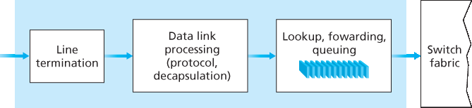
图 4.5 输入端口处理
为了说明如何处理这个规模问题,假设我们的路由器有四个链路,编号为 0 到 3,分组将被转发到以下链路接口:
目的地址范围 |
链路接口 |
|---|---|
11001000 00010111 00010000 00000000 |
0 |
到 |
|
11001000 00010111 00010111 11111111 |
|
11001000 00010111 00011000 00000000 |
1 |
到 |
|
11001000 00010111 00011000 11111111 |
|
11001000 00010111 00011001 00000000 |
2 |
到 |
|
11001000 00010111 00011111 11111111 |
|
其他情况 |
3 |
显然,对于该示例,路由器的转发表无需包含 40 亿条记录。我们可以用如下仅包含四条记录的转发表:
前缀 |
链路接口 |
|---|---|
11001000 00010111 00010 |
0 |
11001000 00010111 00011000 |
1 |
11001000 00010111 00011 |
2 |
其他情况 |
3 |
在这种样式的转发表中,路由器将分组目的地址的 前缀 与表中的条目进行匹配;如果匹配成功,路由器就将分组转发到与匹配项关联的链路。例如,假设分组的目的地址是 11001000 00010111 00010110 10100001;因为该地址的前 21 位前缀匹配表中的第一条记录,路由器将分组转发到链路接口 0。如果前缀不匹配前三条记录中的任何一条,那么路由器就会将分组转发到默认接口 3。尽管这听起来足够简单,但其中有一个非常重要的细节。你可能已经注意到,一个目的地址可能匹配多条记录。例如,地址 11001000 00010111 00011000 10101010 的前 24 位与表中的第二条记录匹配,而其前 21 位与第三条记录匹配。当存在多个匹配时,路由器使用 最长前缀匹配规则;也就是说,路由器找到匹配长度最长的表项,并将分组转发到与该最长前缀匹配项关联的链路接口。当我们在 第 4.3 节 更深入地学习互联网地址时,会进一步解释为何使用最长前缀匹配规则。
在存在转发表的前提下,查找在概念上是简单的——硬件逻辑只需在转发表中搜索最长前缀匹配即可。但在千兆比特传输速率下,查找必须在纳秒级时间内完成(回忆我们之前的例子,一个 10 Gbps 链路与一个 64 字节 IP 数据报)。因此,查找不仅必须通过硬件完成,而且还需使用超越简单线性搜索的大型表的技术;关于快速查找算法的综述可参考 [Gupta 2001, Ruiz-Sanchez 2001]。对内存访问时间也必须特别关注,因此在设计中引入了片上嵌入式 DRAM 以及更快的 SRAM(作为 DRAM 缓存)存储器。实际上,三态内容可寻址存储器(TCAM)也常用于查找 [Yu 2004]。使用 TCAM 时,将 32 位 IP 地址提供给存储器,即可在本质上恒定的时间内返回该地址的转发表项内容。Cisco Catalyst 6500 和 7600 系列的路由器与交换机可以容纳多达一百万条 TCAM 转发表项 [Cisco TCAM 2014]。
一旦通过查找确定了分组的输出端口,该分组就可以被送入交换结构。在某些设计中,如果其他输入端口的分组当前正在使用交换结构,那么某个分组可能会暂时被阻塞,无法进入交换结构。被阻塞的分组将被排队于输入端口,并安排在稍后的时间点穿越交换结构。我们很快将更详细地观察分组的阻塞、排队与调度(在输入端口和输出端口均有)。尽管“查找”可说是输入端口处理中最重要的操作,但还必须执行许多其他操作:(1) 必须执行物理层与链路层处理,如前所述;(2) 必须检查并重写分组的版本号、校验和与生存时间字段,我们将在 第 4.3 节 中学习;(3) 必须更新用于网络管理的计数器(如接收到的 IP 数据报数量)。
我们以一个观点结束输入端口处理的讨论:输入端口查找目的 IP 地址(“匹配”)并将分组送入交换结构到指定输出端口(“动作”)的操作,是一种更通用的“匹配加动作(match plus action)”抽象的具体实现,这种抽象存在于许多网络设备中,而不仅仅是路由器。在链路层交换机中(见 第 6 章),查找链路层目的地址后,除了将帧送入交换结构指向输出端口外,还可能采取其他动作。在防火墙中(见 第 8 章)——这种设备用于过滤特定的入站分组——如果某个入站分组的首部匹配给定条件(例如源/目的 IP 地址和传输层端口号的组合),该分组可能会被丢弃(动作)。在网络地址转换器(NAT,见 第 4.3 节)中,若入站分组的传输层端口号匹配某个值,则在转发前,该分组的端口号将被重写(动作)。确实,“匹配加动作”抽象在当今网络设备中既强大又普遍存在,并且是我们将在 第 4.4 节 中学习的通用转发理念的核心。
A more detailed view of input processing is shown in Figure 4.5. As just discussed, the input port’s line- termination function and link-layer processing implement the physical and link layers for that individual input link. The lookup performed in the input port is central to the router’s operation—it is here that the router uses the forwarding table to look up the output port to which an arriving packet will be forwarded via the switching fabric. The forwarding table is either computed and updated by the routing processor (using a routing protocol to interact with the routing processors in other network routers) or is received from a remote SDN controller. The forwarding table is copied from the routing processor to the line cards over a separate bus (e.g., a PCI bus) indicated by the dashed line from the routing processor to the input line cards in Figure 4.4. With such a shadow copy at each line card, forwarding decisions can be made locally, at each input port, without invoking the centralized routing processor on a per-packet basis and thus avoiding a centralized processing bottleneck.
Let’s now consider the “simplest” case that the output port to which an incoming packet is to be switched is based on the packet’s destination address. In the case of 32-bit IP addresses, a brute-force implementation of the forwarding table would have one entry for every possible destination address. Since there are more than 4 billion possible addresses, this option is totally out of the question.
Figure 4.5 Input port processing
As an example of how this issue of scale can be handled, let’s suppose that our router has four links, numbered 0 through 3, and that packets are to be forwarded to the link interfaces as follows:
Destination Address Range |
Link Interface |
|---|---|
11001000 00010111 00010000 00000000 |
0 |
through |
|
11001000 00010111 00010111 11111111 |
|
11001000 00010111 00011000 00000000 |
1 |
through |
|
11001000 00010111 00011000 11111111 |
|
11001000 00010111 00011001 00000000 |
2 |
through |
|
11001000 00010111 00011111 11111111 |
|
Otherwise |
3 |
Clearly, for this example, it is not necessary to have 4 billion entries in the router’s forwarding table. We could, for example, have the following forwarding table with just four entries:
Prefix |
Link Interface |
|---|---|
11001000 00010111 00010 |
0 |
11001000 00010111 00011000 |
1 |
11001000 00010111 00011 |
2 |
Otherwise |
3 |
With this style of forwarding table, the router matches a prefix of the packet’s destination address with
the entries in the table; if there’s a match, the router forwards the packet to a link associated with the
match. For example, suppose the packet’s destination address is 11001000 00010111 00010110 10100001 ; because the 21-bit prefix of this address matches the first entry in the table, the router
forwards the packet to link interface 0. If a prefix doesn’t match any of the first three entries, then the
router forwards the packet to the default interface 3. Although this sounds simple enough, there’s a very
important subtlety here. You may have noticed that it is possible for a destination address to match
more than one entry. For example, the first 24 bits of the address 11001000 00010111 00011000 10101010 match the second entry in the table, and the first 21 bits of the address match the third entry
in the table. When there are multiple matches, the router uses the longest prefix matching rule; that
is, it finds the longest matching entry in the table and forwards the packet to the link interface associated
with the longest prefix match. We’ll see exactly why this longest prefix-matching rule is used when we
study Internet addressing in more detail in Section 4.3.
Given the existence of a forwarding table, lookup is conceptually simple—hardware logic just searches through the forwarding table looking for the longest prefix match. But at Gigabit transmission rates, this lookup must be performed in nanoseconds (recall our earlier example of a 10 Gbps link and a 64-byte IP datagram). Thus, not only must lookup be performed in hardware, but techniques beyond a simple linear search through a large table are needed; surveys of fast lookup algorithms can be found in [Gupta 2001, Ruiz-Sanchez 2001]. Special attention must also be paid to memory access times, resulting in designs with embedded on-chip DRAM and faster SRAM (used as a DRAM cache) memories. In practice, Ternary Content Addressable Memories (TCAMs) are also often used for lookup [Yu 2004]. With a TCAM, a 32-bit IP address is presented to the memory, which returns the content of the forwarding table entry for that address in essentially constant time. The Cisco Catalyst 6500 and 7600 Series routers and switches can hold upwards of a million TCAM forwarding table entries [Cisco TCAM 2014].
Once a packet’s output port has been determined via the lookup, the packet can be sent into the switching fabric. In some designs, a packet may be temporarily blocked from entering the switching fabric if packets from other input ports are currently using the fabric. A blocked packet will be queued at the input port and then scheduled to cross the fabric at a later point in time. We’ll take a closer look at the blocking, queuing, and scheduling of packets (at both input ports and output ports) shortly. Although “lookup” is arguably the most important action in input port processing, many other actions must be taken: (1) physical- and link-layer processing must occur, as discussed previously; (2) the packet’s version number, checksum and time-to-live field—all of which we’ll study in Section 4.3—must be checked and the latter two fields rewritten; and (3) counters used for network management (such as the number of IP datagrams received) must be updated.
Let’s close our discussion of input port processing by noting that the input port steps of looking up a destination IP address (“match”) and then sending the packet into the switching fabric to the specified output port (“action”) is a specific case of a more general “match plus action” abstraction that is performed in many networked devices, not just routers. In link-layer switches (covered in Chapter 6), link-layer destination addresses are looked up and several actions may be taken in addition to sending the frame into the switching fabric towards the output port. In firewalls (covered in Chapter 8)—devices that filter out selected incoming packets—an incoming packet whose header matches a given criteria (e.g., a combination of source/destination IP addresses and transport-layer port numbers) may be dropped (action). In a network address translator (NAT, covered in Section 4.3), an incoming packet whose transport-layer port number matches a given value will have its port number rewritten before forwarding (action). Indeed, the “match plus action” abstraction is both powerful and prevalent in network devices today, and is central to the notion of generalized forwarding that we’ll study in Section 4.4.
4.2.2 交换#
4.2.2 Switching
交换结构是路由器的核心,因为正是通过该结构,分组才能从输入端口实际交换(即转发)到输出端口。如 图 4.6 所示,交换可以通过多种方式实现:
通过内存交换。最简单、最早的路由器是传统计算机,其输入与输出端口之间的交换由 CPU(路由处理器)直接控制完成。输入端口和输出端口在传统操作系统中作为传统 I/O 设备工作。带有到达分组的输入端口首先通过中断向路由处理器发出信号。然后,该分组被从输入端口复制到处理器内存中。接着,路由处理器从分组首部中提取目的地址,在转发表中查找适当的输出端口,并将分组复制到输出端口的缓冲区。在此情境下,若内存带宽使得每秒最多只能向内存写入或从内存读取 B 个分组,则整体转发吞吐量(即从输入端口到输出端口传输分组的总速率)必须小于 B/2。还要注意,即使两个分组有不同的目的端口,也不能同时被转发,因为共享系统总线上一次只能完成一个内存读写操作。
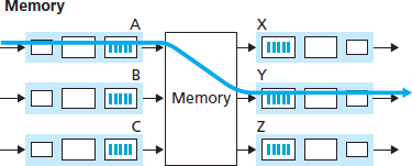
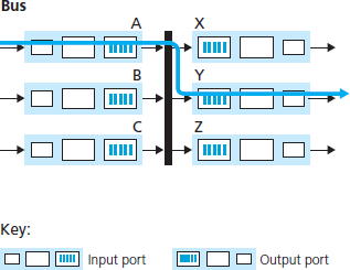
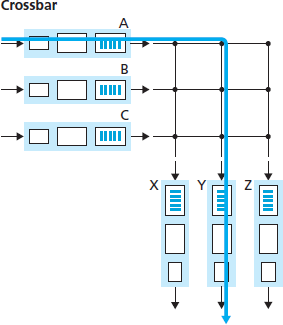
图 4.6 三种交换技术
一些现代路由器通过内存进行交换。然而,与早期路由器的主要区别在于,目的地址的查找与将分组存入适当内存位置的操作是在输入线路卡上的处理器中完成的。在某种意义上,通过内存进行交换的路由器看起来很像共享内存多处理器系统,其中线路卡上的处理单元将分组写入到对应输出端口的内存中。Cisco 的 Catalyst 8500 系列交换机 [Cisco 8500 2016] 内部通过共享内存交换分组。
通过总线交换。在这种方法中,输入端口直接通过共享总线将分组传输到输出端口,无需路由处理器介入。这通常是通过让输入端口在分组前加上一个交换结构内部的标签(首部)实现的,该标签指示该分组将被转发至的本地输出端口,然后将分组发送到总线上。所有输出端口都会接收到该分组,但只有标签匹配的端口会保留该分组。该标签随后在输出端口处被移除,因为它只在交换机内部用于穿越总线。如果多个分组同时到达路由器的不同输入端口,则除了一个外,其余都必须等待,因为每次只能有一个分组穿越总线。由于每个分组都必须穿越单一总线,路由器的交换速率受限于总线速率;在我们的环形交叉口类比中,这就如同该交叉口一次只能容纳一辆车。尽管如此,对于运行在小型局域网和企业网络中的路由器来说,通过总线交换通常已足够。Cisco 6500 路由器 [Cisco 6500 2016] 内部通过 32 Gbps 背板总线交换分组。
通过互连网络交换。克服单个共享总线带宽限制的一种方法是使用更复杂的互连网络,例如过去用于在多处理器计算机架构中互连处理器的网络。交叉开关是一种互连网络,由 2N 条总线组成,连接 N 个输入端口与 N 个输出端口,如 图 4.6 所示。每条垂直总线与每条水平总线在一个交叉点相交,交换结构控制器(其逻辑是交换结构的一部分)可在任意时刻开启或关闭这些交叉点。当一个分组从端口 A 到达并需被转发至端口 Y 时,交换控制器会关闭总线 A 与 Y 的交叉点,然后端口 A 将分组发送到其总线上,而该分组随后仅被总线 Y 接收。请注意,一个来自端口 B 的分组可以同时被转发至端口 X,因为 A 到 Y 与 B 到 X 的分组使用不同的输入与输出总线。因此,与前两种交换方式不同,交叉开关能够并行转发多个分组。交叉开关是 无阻塞 的——只要没有其他分组当前正被转发至同一输出端口,一个分组就不会在转发过程中被阻止。然而,如果来自两个不同输入端口的两个分组目标都是同一输出端口,则其中一个必须在输入端口等待,因为任一总线上一次只能发送一个分组。Cisco 12000 系列交换机 [Cisco 12000 2016] 使用交叉开关网络;Cisco 7600 系列可配置为使用总线或交叉开关 [Cisco 7600 2016]。
更复杂的互连网络使用多级交换元件,使得来自不同输入端口的分组可以同时通过多级交换结构前往同一输出端口。有关交换架构的综述,可参阅 [Tobagi 1990]。Cisco CRS 使用一种三级无阻塞交换策略。路由器的交换容量也可以通过并行运行多个交换结构来扩展。在这种方法中,输入端口与输出端口连接到 N 个并行运行的交换结构。输入端口将一个分组拆分成 K 个较小的块,并通过这 N 个交换结构中的 K 个将这些块“喷射”至所选输出端口,然后该输出端口将这 K 个块重新组装为原始分组。
The switching fabric is at the very heart of a router, as it is through this fabric that the packets are actually switched (that is, forwarded) from an input port to an output port. Switching can be accomplished in a number of ways, as shown in Figure 4.6:
Switching via memory. The simplest, earliest routers were traditional computers, with switching between input and output ports being done under direct control of the CPU (routing processor). Input and output ports functioned as traditional I/O devices in a traditional operating system. An input port with an arriving packet first signaled the routing processor via an interrupt. The packet was then copied from the input port into processor memory. The routing processor then extracted the destination address from the header, looked up the appropriate output port in the forwarding table, and copied the packet to the output port’s buffers. In this scenario, if the memory bandwidth is such that a maximum of B packets per second can be written into, or read from, memory, then the overall forwarding throughput (the total rate at which packets are transferred from input ports to output ports) must be less than B/2. Note also that two packets cannot be forwarded at the same time, even if they have different destination ports, since only one memory read/write can be done at a time over the shared system bus.
Figure 4.6 Three switching techniques
Some modern routers switch via memory. A major difference from early routers, however, is that the lookup of the destination address and the storing of the packet into the appropriate memory location are performed by processing on the input line cards. In some ways, routers that switch via memory look very much like shared-memory multiprocessors, with the processing on a line card switching (writing) packets into the memory of the appropriate output port. Cisco’s Catalyst 8500 series switches [Cisco 8500 2016] internally switches packets via a shared memory.
Switching via a bus. In this approach, an input port transfers a packet directly to the output port over a shared bus, without intervention by the routing processor. This is typically done by having the input port pre-pend a switch-internal label (header) to the packet indicating the local output port to which this packet is being transferred and transmitting the packet onto the bus. All output ports receive the packet, but only the port that matches the label will keep the packet. The label is then removed at the output port, as this label is only used within the switch to cross the bus. If multiple packets arrive to the router at the same time, each at a different input port, all but one must wait since only one packet can cross the bus at a time. Because every packet must cross the single bus, the switching speed of the router is limited to the bus speed; in our roundabout analogy, this is as if the roundabout could only contain one car at a time. Nonetheless, switching via a bus is often sufficient for routers that operate in small local area and enterprise networks. The Cisco 6500 router [Cisco 6500 2016] internally switches packets over a 32-Gbps-backplane bus.
Switching via an interconnection network. One way to overcome the bandwidth limitation of a single, shared bus is to use a more sophisticated interconnection network, such as those that have been used in the past to interconnect processors in a multiprocessor computer architecture. A crossbar switch is an interconnection network consisting of 2N buses that connect N input ports to N output ports, as shown in Figure 4.6. Each vertical bus intersects each horizontal bus at a crosspoint, which can be opened or closed at any time by the switch fabric controller (whose logic ispart of the switching fabric itself). When a packet arrives from port A and needs to be forwarded to port Y, the switch controller closes the crosspoint at the intersection of busses A and Y, and port A then sends the packet onto its bus, which is picked up (only) by bus Y. Note that a packet from port B can be forwarded to port X at the same time, since the A-to-Y and B-to-X packets use different input and output busses. Thus, unlike the previous two switching approaches, crossbar switches are capable of forwarding multiple packets in parallel. A crossbar switch is non-blocking—a packet being forwarded to an output port will not be blocked from reaching that output port as long as no other packet is currently being forwarded to that output port. However, if two packets from two different input ports are destined to that same output port, then one will have to wait at the input, since only one packet can be sent over any given bus at a time. Cisco 12000 series switches [Cisco 12000 2016] use a crossbar switching network; the Cisco 7600 series can be configured to use either a bus or crossbar switch [Cisco 7600 2016].
More sophisticated interconnection networks use multiple stages of switching elements to allow packets from different input ports to proceed towards the same output port at the same time through the multi-stage switching fabric. See [Tobagi 1990] for a survey of switch architectures. The Cisco CRS employs a three-stage non-blocking switching strategy. A router’s switching capacity can also be scaled by running multiple switching fabrics in parallel. In this approach, input ports and output ports are connected to N switching fabrics that operate in parallel. An input port breaks a packet into K smaller chunks, and sends (“sprays”) the chunks through K of these N switching fabrics to the selected output port, which reassembles the K chunks back into the original packet.
4.2.3 输出端口处理#
4.2.3 Output Port Processing
输出端口处理如 图 4.7 所示,它将已经存储在输出端口内存中的分组通过输出链路进行传输。这包括为传输选择并出队分组,以及执行所需的链路层和物理层传输功能。
Output port processing, shown in Figure 4.7, takes packets that have been stored in the output port’s memory and transmits them over the output link. This includes selecting and de-queueing packets for transmission, and performing the needed link-layer and physical-layer transmission functions.
4.2.4 排队发生在哪里?#
4.2.4 Where Does Queuing Occur?
如果我们考虑输入端口和输出端口的功能以及 图 4.6 所示的配置,很明显,在输入端口和输出端口都可能形成分组队列,就像我们在环形交叉口类比中识别出汽车可能在交叉口的入口和出口处等待一样。排队的位置与程度(无论是在输入端口队列还是输出端口队列)将取决于流量负载、交换结构的相对速度以及链路速度。现在我们将更详细地考虑这些队列,因为当这些队列变得很大时,路由器的内存最终可能被耗尽,并在没有可用内存来存储到达的分组时发生 分组丢失。回想我们之前的讨论,我们曾说过分组“在网络中丢失”或“在路由器处被丢弃”。 正是在路由器中的这些队列中,这些分组实际上被丢弃和丢失 。
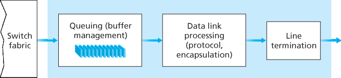
图 4.7 输出端口处理
假设输入和输出链路的传输速率均为 \(R_{line}\) 个分组每秒,并且有 N 个输入端口和 N 个输出端口。为了进一步简化讨论,假设所有分组长度相同,且分组以同步方式到达输入端口。也就是说,在任何链路上发送一个分组所需的时间等于在任何链路上接收一个分组所需的时间,并且在这段时间间隔内,每条输入链路上只能到达零个或一个分组。将交换结构的传输速率定义为 \(R_{switch}\),即分组可以从输入端口传送到输出端口的速率。如果 \(R_{switch}\) 是 \(R_{line}\) 的 N 倍,则在输入端口处几乎不会发生排队。这是因为即使在最坏情况下,即所有 N 条输入链路都在接收分组,且所有分组都要转发至同一输出端口,每一批 N 个分组(每个输入端口一个分组)也可以在下一批到达前通过交换结构完成传输。
If we consider input and output port functionality and the configurations shown in Figure 4.6, it’s clear that packet queues may form at both the input ports and the output ports, just as we identified cases where cars may wait at the inputs and outputs of the traffic intersection in our roundabout analogy. The location and extent of queueing (either at the input port queues or the output port queues) will depend on the traffic load, the relative speed of the switching fabric, and the line speed. Let’s now consider these queues in a bit more detail, since as these queues grow large, the router’s memory can eventually be exhausted and packet loss will occur when no memory is available to store arriving packets. Recall that in our earlier discussions, we said that packets were “lost within the network” or “dropped at a router.” It is here, at these queues within a router, where such packets are actually dropped and lost.
Figure 4.7 Output port processing
Suppose that the input and output line speeds (transmission rates) all have an identical transmission rate of \(R_{line}\) packets per second, and that there are N input ports and N output ports. To further simplify the discussion, let’s assume that all packets have the same fixed length, and that packets arrive to input ports in a synchronous manner. That is, the time to send a packet on any link is equal to the time to receive a packet on any link, and during such an interval of time, either zero or one packets can arrive on an input link. Define the switching fabric transfer rate \(R_{switch}\) as the rate at which packets can be moved from input port to output port. If \(R_{switch}\) is N times faster than \(R_{line}\), then only negligible queuing will occur at the input ports. This is because even in the worst case, where all N input lines are receiving packets, and all packets are to be forwarded to the same output port, each batch of N packets (one packet per input port) can be cleared through the switch fabric before the next batch arrives.
输入排队#
Input Queueing
但如果交换结构的速度不足(相对于输入链路速率)以无延迟地传送所有到达的分组会发生什么?在这种情况下,输入端口也会发生分组排队,因为分组必须加入输入端口队列,等待它们被传送通过交换结构到输出端口。为了说明这种排队所带来的一个重要后果,考虑一个交叉开关结构,并假设:(1)所有链路速率相同;(2)从任一输入端口向给定输出端口传送一个分组所需的时间与在输入链路上接收一个分组所需的时间相同;(3)分组从给定输入队列按 FCFS(先进先出)方式转移至其期望的输出队列。只要它们的输出端口不同,就可以并行转发多个分组。然而,如果两个输入队列前端的分组目标是同一输出队列,则其中一个分组将被阻塞,必须在输入队列中等待——因为交换结构一次只能将一个分组传送至某一给定输出端口。
图 4.8 展示了一个示例,其中两个输入队列前端的分组(深色阴影)目标是同一个右上角输出端口。假设交换结构选择传送左上角队列前端的分组。在这种情况下,左下角队列中的深色分组必须等待。但不仅该深色分组必须等待,其后排队的浅色分组也必须等待,即使该浅色分组的目的地是中间右侧的输出端口(没有冲突)。这种现象称为 队头阻塞(HOL blocking),即在输入排队交换机中,输入队列中的一个排队分组必须等待被交换结构传输(即使其输出端口是空闲的),因为它被队列最前端的另一个分组所阻塞。[Karol 1987] 表明,在某些假设下,当输入链路上的分组到达率仅达到其容量的 58% 时,由于队头阻塞,输入队列长度将增长至无界(非正式地说,这等价于显著的分组丢失将会发生)。解决队头阻塞的多种方案将在 [McKeown 1997] 中讨论。
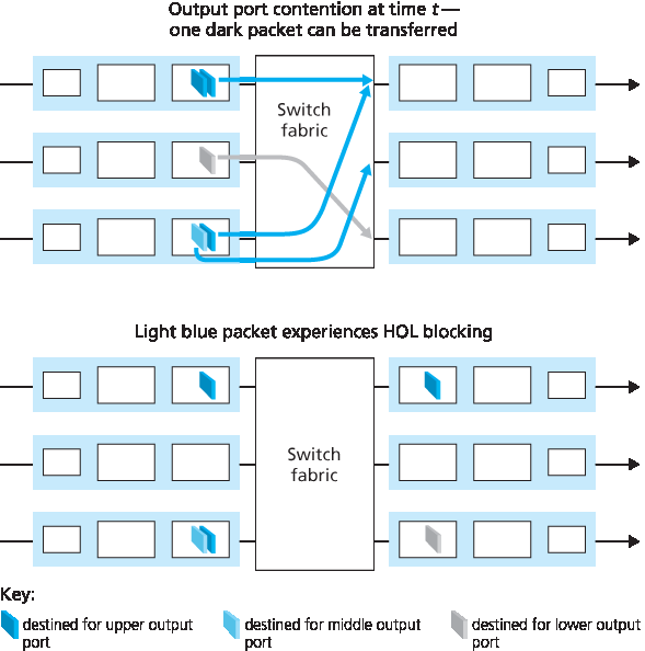
图 4.8 输入排队交换机中的队头阻塞(HOL blocking)
But what happens if the switch fabric is not fast enough (relative to the input line speeds) to transfer all arriving packets through the fabric without delay? In this case, packet queuing can also occur at the input ports, as packets must join input port queues to wait their turn to be transferred through the switching fabric to the output port. To illustrate an important consequence of this queuing, consider a crossbar switching fabric and suppose that (1) all link speeds are identical, (2) that one packet can be transferred from any one input port to a given output port in the same amount of time it takes for a packet to be received on an input link, and (3) packets are moved from a given input queue to their desired output queue in an FCFS manner. Multiple packets can be transferred in parallel, as long as their output ports are different. However, if two packets at the front of two input queues are destined for the same output queue, then one of the packets will be blocked and must wait at the input queue—the switching fabric can transfer only one packet to a given output port at a time.
Figure 4.8 shows an example in which two packets (darkly shaded) at the front of their input queues are destined for the same upper-right output port. Suppose that the switch fabric chooses to transfer the packet from the front of the upper-left queue. In this case, the darkly shaded packet in the lower-left queue must wait. But not only must this darkly shaded packet wait, so too must the lightly shadedpacket that is queued behind that packet in the lower-left queue, even though there is no contention for the middle-right output port (the destination for the lightly shaded packet). This phenomenon is known as head-of-the-line (HOL) blocking in an input-queued switch—a queued packet in an input queue must wait for transfer through the fabric (even though its output port is free) because it is blocked by another packet at the head of the line. [Karol 1987] shows that due to HOL blocking, the input queue will grow to unbounded length (informally, this is equivalent to saying that significant packet loss will occur) under certain assumptions as soon as the packet arrival rate on the input links reaches only 58 percent of their capacity. A number of solutions to HOL blocking are discussed in [McKeown 1997].
Figure 4.8 HOL blocking at and input-queued switch
输出排队#
Output Queueing
接下来我们来考虑在交换机的输出端口是否也会发生排队。假设 \(R_{switch}\) 再次是 \(R_{line}\) 的 N 倍,并且到达每个 N 个输入端口的分组都要发往同一个输出端口。在这种情况下,在将一个分组发送到输出链路所需的时间内,会有 N 个新的分组到达该输出端口(每个输入端口一个分组)。由于输出端口在一个单位时间(即分组的传输时间)内只能发送一个分组,因此这 N 个到达的分组必须排队等待通过输出链路进行传输。然后,在仅仅传输这 N 个排队分组中的一个所需的时间内,可能又会有 N 个分组到达。以此类推。因此,即使交换结构的速率是端口链路速率的 N 倍,输出端口也可能形成分组队列。最终,排队的分组数量可能增长到足以耗尽输出端口的可用内存。
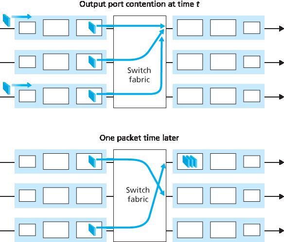
图 4.9 输出端口排队
当没有足够的内存来缓冲一个到达的分组时,必须做出一个决定:是丢弃该到达的分组(这一策略称为 尾部丢弃(drop-tail)),还是移除一个或多个已经排队的分组,以为新到达的分组腾出空间。在某些情况下,在缓冲区满之前丢弃(或标记)一个分组可能是有利的,这样可以向发送方提供拥塞信号。一些积极主动的分组丢弃与标记策略(统称为 主动队列管理(AQM) 算法)已被提出和分析 [Labrador 1999, Hollot 2002]。最广为研究和实现的 AQM 算法之一是 随机早期检测(RED) 算法 [Christiansen 2001; Floyd 2016]。
输出端口排队如 图 4.9 所示。在时间 t,每个输入端口上都有一个分组到达,并且都目标为最上方的输出端口。假设链路速率相同,且交换机以三倍于链路速率的速率运行,在一个时间单位后(也就是接收或发送一个分组所需的时间),这三个原始分组都已经被转发到输出端口,并排队等待传输。在下一个时间单位中,这三个分组中的一个已经通过输出链路传输。在我们的示例中,又有两个新分组到达交换机输入端,其中一个目标为最上方的输出端口。这种排队的一个后果是,输出端口上的一个 分组调度器 必须从排队的分组中选择一个用于传输 —— 这是我们将在下一节中介绍的主题。
考虑到路由器缓冲区的作用是吸收流量负载的波动,一个自然的问题是到底需要多少缓冲空间。多年来,[RFC 3439] 中的经验法则认为,缓冲大小(B)应等于平均往返时间(RTT,假设为 250 毫秒)乘以链路容量(C)。这个结果基于对相对较少 TCP 流的排队动态分析 [Villamizar 1994]。因此,对于一条 10 Gbps 链路和 250 毫秒的 RTT,所需缓冲空间为 B = RTT · C = 2.5 Gbit。更近期的理论与实验研究 [Appenzeller 2004] 表明,当有大量 TCP 流(N)通过某条链路时,所需的缓冲空间为 B = RTT · C / N。在大型骨干路由器链路上传输的 TCP 流数量通常很大(见例如 [Fraleigh 2003]),N 值可以非常大,从而显著降低所需的缓冲大小。[[Appenzeller 2004]; Wischik 2005; Beheshti 2008] 对缓冲大小问题从理论、实现与运维角度提供了易读性很强的讨论。
Let’s next consider whether queueing can occur at a switch’s output ports. Suppose that \(R_{switch}\) is again N times faster than \(R_{line}\) and that packets arriving at each of the N input ports are destined to the same output port. In this case, in the time it takes to send a single packet onto the outgoing link, N new packets will arrive at this output port (one from each of the N input ports). Since the output port cantransmit only a single packet in a unit of time (the packet transmission time), the N arriving packets will have to queue (wait) for transmission over the outgoing link. Then N more packets can possibly arrive in the time it takes to transmit just one of the N packets that had just previously been queued. And so on. Thus, packet queues can form at the output ports even when the switching fabric is N times faster than the port line speeds. Eventually, the number of queued packets can grow large enough to exhaust available memory at the output port.
Figure 4.9 Output port queueing
When there is not enough memory to buffer an incoming packet, a decision must be made to either drop the arriving packet (a policy known as drop-tail) or remove one or more already-queued packets to make room for the newly arrived packet. In some cases, it may be advantageous to drop (or mark the header of) a packet before the buffer is full in order to provide a congestion signal to the sender. A number of proactive packet-dropping and -marking policies (which collectively have become known as active queue management (AQM) algorithms) have been proposed and analyzed [Labrador 1999, Hollot 2002]. One of the most widely studied and implemented AQM algorithms is the Random Early Detection (RED) algorithm [Christiansen 2001; Floyd 2016].
Output port queuing is illustrated in Figure 4.9. At time t, a packet has arrived at each of the incoming input ports, each destined for the uppermost outgoing port. Assuming identical line speeds and a switch operating at three times the line speed, one time unit later (that is, in the time needed to receive or senda packet), all three original packets have been transferred to the outgoing port and are queued awaiting transmission. In the next time unit, one of these three packets will have been transmitted over the outgoing link. In our example, two new packets have arrived at the incoming side of the switch; one of these packets is destined for this uppermost output port. A consequence of such queuing is that a packet scheduler at the output port must choose one packet, among those queued, for transmission— a topic we’ll cover in the following section.
Given that router buffers are needed to absorb the fluctuations in traffic load, a natural question to ask is how much buffering is required. For many years, the rule of thumb [RFC 3439] for buffer sizing was that the amount of buffering (B) should be equal to an average round-trip time (RTT, say 250 msec) times the link capacity (C). This result is based on an analysis of the queueing dynamics of a relatively small number of TCP flows [Villamizar 1994]. Thus, a 10 Gbps link with an RTT of 250 msec would need an amount of buffering equal to B 5 RTT · C 5 2.5 Gbits of buffers. More recent theoretical and experimental efforts [Appenzeller 2004], however, suggest that when there are a large number of TCP flows (N) passing through a link, the amount of buffering needed is B=RTI⋅C/N. With a large number of flows typically passing through large backbone router links (see, e.g., [Fraleigh 2003]), the value of N can be large, with the decrease in needed buffer size becoming quite significant. [[Appenzeller 2004]; Wischik 2005; Beheshti 2008] provide very readable discussions of the buffer-sizing problem from a theoretical, implementation, and operational standpoint.
4.2.5 分组调度#
4.2.5 Packet Scheduling
现在我们回到之前的问题,即如何确定排队分组在输出链路上的传输顺序。你自己无疑曾多次排过长队,并观察过等候顾客是如何被服务的,因此你一定很熟悉路由器中常用的各种排队策略。有先来先服务(FCFS,也称为先进先出,FIFO)。英国人以在公交车站和市场中有耐心、守秩序地排 FIFO 队而闻名(“哦,你是在排队吗?”)。其他国家则采用优先级方式服务,某一类等候顾客会被优先服务于其他顾客。还有轮询排队方式,即顾客被分成不同的类别(如同优先队列中那样),但各类顾客轮流接受服务。
Let’s now return to the question of determining the order in which queued packets are transmitted over an outgoing link. Since you yourself have undoubtedly had to wait in long lines on many occasions and observed how waiting customers are served, you’re no doubt familiar with many of the queueing disciplines commonly used in routers. There is first-come-first-served (FCFS, also known as first-in-first- out, FIFO). The British are famous for patient and orderly FCFS queueing at bus stops and in the marketplace (“Oh, are you queueing?”). Other countries operate on a priority basis, with one class of waiting customers given priority service over other waiting customers. There is also round-robin queueing, where customers are again divided into classes (as in priority queueing) but each class of customer is given service in turn.
先进先出(FIFO)#
First-in-First-Out (FIFO)
图 4.10 展示了用于 FIFO 链路调度策略的排队模型抽象。当输出链路正忙于传输另一个分组时,到达的分组将在链路的输出队列中等待传输。如果没有足够的缓冲空间来存储到达的分组,那么队列的丢弃策略将决定该分组是否被丢弃(丢失),或者是否从队列中移除其他分组以为该到达分组腾出空间,如上所述。在下面的讨论中,我们将忽略分组丢弃的情形。当一个分组完全通过输出链路传输(即“获得服务”)后,它就从队列中移除。
FIFO(也称为先来先服务,FCFS)调度策略按分组到达输出队列的顺序选择分组进行链路传输。我们都熟悉服务中心中的 FIFO 排队方式,到达的顾客排在队列尾部,按顺序等待,最终在排到前面时获得服务。图 4.11 展示了 FIFO 队列的工作方式。分组到达由上方时间线上的编号箭头表示,编号表示分组到达的顺序。各个分组的离开则在下方时间线上标出。分组正在传输期间的时间由两条时间线之间的阴影矩形表示。在我们的示例中,假设每个分组需要 3 个时间单位传输。在 FIFO 策略下,分组按它们到达的顺序离开。注意,在分组 4 离开后,由于分组 1 到 4 已经传输完毕并被从队列中移除,链路在分组 5 到达之前将保持空闲状态。
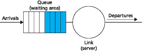
图 4.10 FIFO 排队抽象
Figure 4.10 shows the queuing model abstraction for the FIFO link-scheduling discipline. Packets arriving at the link output queue wait for transmission if the link is currently busy transmitting another packet. If there is not sufficient buffering space to hold the arriving packet, the queue’s packet- discarding policy then determines whether the packet will be dropped (lost) or whether other packets will be removed from the queue to make space for the arriving packet, as discussed above. In ourdiscussion below, we’ll ignore packet discard. When a packet is completely transmitted over the outgoing link (that is, receives service) it is removed from the queue.
The FIFO (also known as first-come-first-served, or FCFS) scheduling discipline selects packets for link transmission in the same order in which they arrived at the output link queue. We’re all familiar with FIFO queuing from service centers, where arriving customers join the back of the single waiting line, remain in order, and are then served when they reach the front of the line. Figure 4.11 shows the FIFO queue in operation. Packet arrivals are indicated by numbered arrows above the upper timeline, with the number indicating the order in which the packet arrived. Individual packet departures are shown below the lower timeline. The time that a packet spends in service (being transmitted) is indicated by the shaded rectangle between the two timelines. In our examples here, let’s assume that each packet takes three units of time to be transmitted. Under the FIFO discipline, packets leave in the same order in which they arrived. Note that after the departure of packet 4, the link remains idle (since packets 1 through 4 have been transmitted and removed from the queue) until the arrival of packet 5.
Figure 4.10 FIFO queueing abstraction
优先级排队#
Priority Queuing
在优先级排队中,到达输出链路的分组在到达队列时被分类为不同的优先级类别,如 图 4.12 所示。在实际中,网络运营商可能会配置队列,使得携带网络管理信息的分组(例如,通过 TCP/UDP 源端口或目的端口号标识)相对于用户流量获得更高的优先级;此外,实时语音(如 VoIP)分组可能相对于非实时流量(如 SMTP 或 IMAP 邮件分组)具有更高优先级。每个优先级类别通常拥有其自己的队列。当选择要传输的分组时,优先级排队策略将从具有非空队列的最高优先级类别中传输一个分组(即,有待传输分组)。在相同优先级类别内的分组选择通常采用 FIFO 方式。
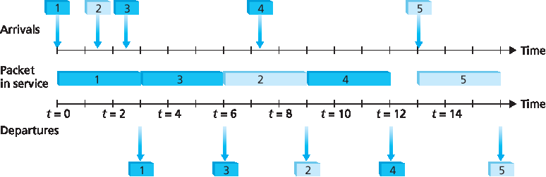
图 4.13 优先级队列的运行方式
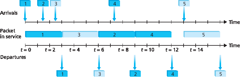
图 4.14 两类轮询队列的运行方式
图 4.13 展示了一个包含两个优先级类别的优先级队列的运行过程。分组 1、3 和 4 属于高优先级类别,分组 2 和 5 属于低优先级类别。分组 1 到达后发现链路空闲,立即开始传输。在分组 1 传输期间,分组 2 和 3 到达,分别进入低优先级和高优先级队列。在分组 1 传输完成后,分组 3(高优先级)被选中传输,而不是分组 2(尽管其更早到达,但为低优先级)。分组 3 传输结束后,分组 2 才开始传输。分组 4(高优先级)在分组 2(低优先级)传输期间到达。在 非抢占式优先级排队 策略中,一旦某个分组开始传输,其传输将不会被中断。在这种情况下,分组 4 会进入排队等待,并在分组 2 传输完成后开始传输。
Under priority queuing, packets arriving at the output link are classified into priority classes upon arrival at the queue, as shown in Figure 4.12. In practice, a network operator may configure a queue so that packets carrying network management information (e.g., as indicated by the source or destination TCP/UDP port number) receive priority over user traffic; additionally, real-time voice-over-IP packets might receive priority over non-real traffic such as SMTP or IMAP e-mail packets. Each priority class typically has its own queue. When choosing a packet to transmit, the priority queuing discipline will transmit a packet from the highest priority class that has a nonempty queue (that is, has packets waiting for transmission). The choice among packets in the same priority class is typically done in a FIFO manner.
Figure 4.13 The priority queue in operation
Figure 4.14 The two-class robin queue in operation
Figure 4.13 illustrates the operation of a priority queue with two priority classes. Packets 1, 3, and 4 belong to the high-priority class, and packets 2 and 5 belong to the low-priority class. Packet 1 arrives and, finding the link idle, begins transmission. During the transmission of packet 1, packets 2 and 3 arrive and are queued in the low- and high-priority queues, respectively. After the transmission of packet 1, packet 3 (a high-priority packet) is selected for transmission over packet 2 (which, even though it arrived earlier, is a low-priority packet). At the end of the transmission of packet 3, packet 2 then begins transmission. Packet 4 (a high-priority packet) arrives during the transmission of packet 2 (a low-priority packet). Under a non-preemptive priority queuing discipline, the transmission of a packet is not interrupted once it has begun. In this case, packet 4 queues for transmission and begins being transmitted after the transmission of packet 2 is completed.
轮询与加权公平排队(WFQ)#
Round Robin and Weighted Fair Queuing (WFQ)
在轮询排队策略中,分组和优先级排队一样被分为多个类别。然而,不同类别之间并不具有严格的服务优先级,而是由轮询调度器轮流为各类分组服务。在最简单的轮询调度中,传输一个类别 1 的分组,接着传输一个类别 2 的分组,再传输一个类别 1 的分组,之后是类别 2 的分组,如此交替进行。所谓的 工作保持型排队 策略只要队列中有任何类别的分组待传输,就不会让链路保持空闲。一个工作保持型的轮询策略在查找某一类分组未果时,会立即检查下一类别。
图 4.14 展示了一个两类轮询队列的运行过程。在该示例中,分组 1、2 和 4 属于类别 1,分组 3 和 5 属于类别 2。分组 1 到达输出队列后立即开始传输。分组 2 和 3 在分组 1 传输期间到达,因此被排入队列。分组 1 传输完成后,链路调度器查找类别 2 的分组,因此传输了分组 3。分组 3 传输完成后,调度器查找类别 1 的分组,因此传输了分组 2。分组 2 传输完成后,分组 4 是唯一排队的分组,因此立即被传输。
一种在路由器中广泛实现的轮询排队推广形式是所谓的 加权公平排队(WFQ)策略 [Demers 1990; Parekh 1993; Cisco QoS 2016]。WFQ 如 图 4.15 所示。在此,分组在到达时被分类并排入相应类别的等待区域。与轮询调度一样,WFQ 调度器以循环方式为各类分组服务 —— 先服务类别 1,再服务类别 2,再服务类别 3,然后(假设总共有三个类别)重复这一服务模式。WFQ 也是一种工作保持型排队策略,因此在发现当前类别队列为空时,会立即转向服务序列中的下一个类别。
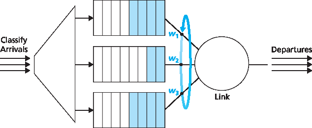
图 4.15 加权公平排队
WFQ 与轮询的不同之处在于,每个类别在任意时间间隔内可以获得不同数量的服务。具体地说,每个类别 i 被赋予一个权重 wi。在 WFQ 中,在任何一个类别 i 有分组待发送的时间段内,该类别将被保证获得一部分服务,其比例为 wi/(∑wj),其中分母中的求和是对所有同样有待传输分组的类别进行的。在最坏的情况下,即使所有类别都有分组排队,类别 i 也仍然能获得至少 wi/(∑wj) 的带宽份额,其中分母中的求和是对所有类别进行的。因此,对于一条传输速率为 R 的链路,类别 i 将始终至少获得 R⋅wi/(∑wj) 的吞吐量。我们对 WFQ 的描述是理想化的,因为我们没有考虑分组是离散的,且某个分组的传输一旦开始,不会被中断以传输另一个分组;[Demers 1990; Parekh 1993] 讨论了这一分组化问题。
Under the round robin queuing discipline, packets are sorted into classes as with priority queuing. However, rather than there being a strict service priority among classes, a round robin scheduler alternates service among the classes. In the simplest form of round robin scheduling, a class 1 packet is transmitted, followed by a class 2 packet, followed by a class 1 packet, followed by a class 2 packet, and so on. A so-called work-conserving queuing discipline will never allow the link to remain idle whenever there are packets (of any class) queued for transmission. A work-conserving round robin discipline that looks for a packet of a given class but finds none will immediately check the next class in the round robin sequence.
Figure 4.14 illustrates the operation of a two-class round robin queue. In this example, packets 1, 2, and4 belong to class 1, and packets 3 and 5 belong to the second class. Packet 1 begins transmission immediately upon arrival at the output queue. Packets 2 and 3 arrive during the transmission of packet 1 and thus queue for transmission. After the transmission of packet 1, the link scheduler looks for a class 2 packet and thus transmits packet 3. After the transmission of packet 3, the scheduler looks for a class 1 packet and thus transmits packet 2. After the transmission of packet 2, packet 4 is the only queued packet; it is thus transmitted immediately after packet 2.
A generalized form of round robin queuing that has been widely implemented in routers is the so-called weighted fair queuing (WFQ) discipline [Demers 1990; Parekh 1993; Cisco QoS 2016]. WFQ is illustrated in Figure 4.15. Here, arriving packets are classified and queued in the appropriate per-class waiting area. As in round robin scheduling, a WFQ scheduler will serve classes in a circular manner— first serving class 1, then serving class 2, then serving class 3, and then (assuming there are three classes) repeating the service pattern. WFQ is also a work-conserving queuing discipline and thus will immediately move on to the next class in the service sequence when it finds an empty class queue.
Figure 4.15 Weighted fair queueing
WFQ differs from round robin in that each class may receive a differential amount of service in any interval of time. Specifically, each class, i, is assigned a weight, wi. Under WFQ, during any interval of time during which there are class i packets to send, class i will then be guaranteed to receive a fraction of service equal to wi/(∑wj), where the sum in the denominator is taken over all classes that also have packets queued for transmission. In the worst case, even if all classes have queued packets, class i will still be guaranteed to receive a fraction wi/(∑wj) of the bandwidth, where in this worst case the sum in the denominator is over all classes. Thus, for a link with transmission rate R, class i will always achieve a throughput of at least R⋅wi/(∑wj). Our description of WFQ has been idealized, as we have not considered the fact that packets are discrete and a packet’s transmission will not be interrupted to begin transmission of another packet; [Demers 1990; Parekh 1993] discuss this packetization issue.