3.6 拥塞控制原理#
3.6 Principles of Congestion Control
在前面的章节中,我们考察了在丢包情况下提供可靠数据传输服务的一般原理和具体的 TCP 机制。我们之前提到,在实际中,这种丢包通常是由于网络拥塞导致路由器缓冲区溢出引起的。因此,分组重传只是处理了网络拥塞的一个症状(即特定传输层报文段的丢失),但并未解决网络拥塞的根本原因——过多的发送方尝试以过高的速率发送数据。要解决网络拥塞的根本原因,就需要在网络拥塞时对发送方进行节流控制。
本节我们在更一般的背景下考虑拥塞控制问题,旨在理解为什么拥塞是坏事,网络拥塞如何表现为上层应用所感知的性能下降,以及为避免或应对网络拥塞可采取的各种方法。由于拥塞控制与可靠数据传输一样,是网络中根本性的重要问题之一,本节对其进行更为广泛的研究。下一节将详细研究 TCP 的拥塞控制算法。
In the previous sections, we examined both the general principles and specific TCP mechanisms used to provide for a reliable data transfer service in the face of packet loss. We mentioned earlier that, in practice, such loss typically results from the overflowing of router buffers as the network becomes congested. Packet retransmission thus treats a symptom of network congestion (the loss of a specific transport-layer segment) but does not treat the cause of network congestion—too many sources attempting to send data at too high a rate. To treat the cause of network congestion, mechanisms are needed to throttle senders in the face of network congestion.
In this section, we consider the problem of congestion control in a general context, seeking to understand why congestion is a bad thing, how network congestion is manifested in the performance received by upper-layer applications, and various approaches that can be taken to avoid, or react to, network congestion. This more general study of congestion control is appropriate since, as with reliable data transfer, it is high on our “top-ten” list of fundamentally important problems in networking. The following section contains a detailed study of TCP’s congestion-control algorithm.
3.6.1 拥塞的原因与代价#
3.6.1 The Causes and the Costs of Congestion
我们从三个越来越复杂的拥塞场景开始一般性的拥塞控制研究。每种情况下,我们都将探讨拥塞产生的原因以及拥塞的代价(资源未充分利用和终端系统收到的性能下降)。我们暂时不关注如何反应或避免拥塞,而是关注当主机提高传输速率且网络变得拥塞时会发生什么。
Let’s begin our general study of congestion control by examining three increasingly complex scenarios in which congestion occurs. In each case, we’ll look at why congestion occurs in the first place and at the cost of congestion (in terms of resources not fully utilized and poor performance received by the end systems). We’ll not (yet) focus on how to react to, or avoid, congestion but rather focus on the simpler issue of understanding what happens as hosts increase their transmission rate and the network becomes congested.
场景1:两个发送方,路由器具有无限缓冲区#
Scenario 1: Two Senders, a Router with Infinite Buffers
我们先考虑可能最简单的拥塞场景:两个主机(A 和 B)各有一个连接,它们共享源与目的地之间的单跳,如 图3.43 所示。
假设主机 A 中的应用以平均速率 λin 字节/秒向连接发送数据(例如,通过套接字向传输层协议传递数据)。这些数据是原始数据,即每个数据单位只被发送一次。底层传输层协议很简单,数据被封装后发送;不执行错误恢复(如重传)、流量控制或拥塞控制。忽略添加传输层和下层头部信息带来的额外开销,则主机 A 在本场景中向路由器提供的流量速率为 λin 字节/秒。主机 B 以类似方式操作,且为简化起见,我们假设它也以 λin 字节/秒的速率发送数据。主机 A 和 B 的分组通过路由器并经过容量为 R 的共享输出链路。路由器具有缓冲区,可以在分组到达速率超过链路容量时暂存分组。在本场景中,假设路由器缓冲区大小无限。
图3.44 绘制了主机 A 连接在本场景下的性能。左图绘制了 每连接吞吐量 (接收端每秒字节数)与连接发送速率的函数关系。对于发送速率在 0 到 R/2 之间,接收端吞吐量等于发送速率——发送方发送的所有数据都以有限延迟被接收。发送速率超过 R/2 时,吞吐量仅为 R/2。吞吐量的这一上限是因为两个连接共享链路容量导致的。链路无法以稳定状态速率向接收端传送超过 R/2 的分组。不论主机 A 和 B 将发送速率设置多高,各自看到的吞吐量均不会超过 R/2。
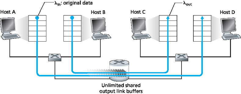
图 3.43 拥塞场景1:两个连接共享单跳且缓冲区无限
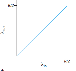
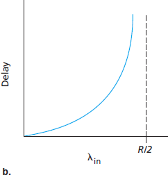
图 3.44 拥塞场景1:吞吐量与延迟随主机发送速率变化
实现每连接吞吐量 R/2 看似是好事,因为链路已被充分利用以传送分组。但 图3.44 右图展示了接近链路容量运作的后果。当发送速率从左侧逼近 R/2 时,平均延迟越来越大。发送速率超过 R/2 时,路由器中排队的分组数无界,源到目的地的平均延迟变为无限(假设连接以该发送速率无限期运行且缓冲无限)。因此,虽然从吞吐角度看近似达到总吞吐 R 是理想的,但从延迟角度看则远非理想。即使在这一极端理想化场景中,我们也已发现网络拥塞的一项代价——当分组到达速率接近链路容量时,经历较大的排队延迟。
We begin by considering perhaps the simplest congestion scenario possible: Two hosts (A and B) each have a connection that shares a single hop between source and destination, as shown in Figure 3.43.
Let’s assume that the application in Host A is sending data into the connection (for example, passing data to the transport-level protocol via a socket) at an average rate of λin bytes/sec. These data are original in the sense that each unit of data is sent into the socket only once. The underlying transport- level protocol is a simple one. Data is encapsulated and sent; no error recovery (for example, retransmission), flow control, or congestion control is performed. Ignoring the additional overhead due to adding transport- and lower-layer header information, the rate at which Host A offers traffic to the router in this first scenario is thus λin bytes/sec. Host B operates in a similar manner, and we assume for simplicity that it too is sending at a rate of λin bytes/sec. Packets from Hosts A and B pass through a router and over a shared outgoing link of capacity R. The router has buffers that allow it to store incoming packets when the packet-arrival rate exceeds the outgoing link’s capacity. In this first scenario, we assume that the router has an infinite amount of buffer space.
Figure 3.44 plots the performance of Host A’s connection under this first scenario. The left graph plots the per-connection throughput (number of bytes per second at the receiver) as a function of the connection-sending rate. For a sending rate between 0 and R/2, the throughput at the receiver equals the sender’s sending rate—everything sent by the sender is received at the receiver with a finite delay. When the sending rate is above R/2, however, the throughput is only R/2. This upper limit on throughput is a consequence of the sharing of link capacity between two connections. The link simply cannot deliver packets to a receiver at a steady-state rate that exceeds R/2. No matter how high Hosts A and B set their sending rates, they will each never see a throughput higher than R/2.
Figure 3.43 Congestion scenario 1: Two connections sharing a single hop with infinite buffers
Figure 3.44 Congestion scenario 1: Throughput and delay as a function of host sending rate
Achieving a per-connection throughput of R/2 might actually appear to be a good thing, because the link is fully utilized in delivering packets to their destinations. The right-hand graph in Figure 3.44, however, shows the consequence of operating near link capacity. As the sending rate approaches R/2 (from the left), the average delay becomes larger and larger. When the sending rate exceeds R/2, the average number of queued packets in the router is unbounded, and the average delay between source and destination becomes infinite (assuming that the connections operate at these sending rates for an infinite period of time and there is an infinite amount of buffering available). Thus, while operating at an aggregate throughput of near R may be ideal from a throughput standpoint, it is far from ideal from a delay standpoint. Even in this (extremely) idealized scenario, we’ve already found one cost of a congested network—large queuing delays are experienced as the packet-arrival rate nears the link capacity.
场景2:两个发送方,路由器缓冲有限#
Scenario 2: Two Senders and a Router with Finite Buffers
现在稍作修改场景1中的两个方面(见 图3.45)。首先,假设路由器缓冲区大小有限。这一现实假设导致当缓冲区已满时到达的分组会被丢弃。其次,假设每个连接是可靠的。如果传输层报文段所在分组在路由器被丢弃,发送方最终会重传。由于可能重传,我们需要更仔细地使用发送速率一词。具体来说,令应用向套接字发送原始数据的速率仍记为 λin 字节/秒。传输层向网络发送(包含原始数据和重传数据)的报文段速率记为 λ′in 字节/秒。λ′in 有时称为网络的 负载输入。
图 3.45 场景2:两个主机(含重传)与有限缓冲路由器
场景2的性能强烈依赖于重传的方式。先考虑不现实的情况,主机 A 能神奇地判断路由器缓冲区是否空闲,只有缓冲空闲时才发送分组。在此情况下,无分组丢失,λin 等于 λ′in,连接吞吐量等于 λin。该情况见 图3.46(a)。从吞吐角度看性能理想——发送即全部接收。注意在此场景下平均主机发送速率不能超过 R/2,因为假设无分组丢失。
再考虑稍微现实的情况,发送方只有在确定分组丢失时才重传。(该假设仍有些牵强,但发送主机可以设置足够长的超时以几乎确保未被确认的分组确实丢失。)此时性能大致如 图3.46(b) 所示。理解这一现象,考虑负载输入 λ′in(原始数据加重传数据速率)等于 R/2 的情况。根据 图3.46(b),此时数据传递给接收应用的速率为 R/3。因此,在发送的 0.5R 单位数据中,平均有 0.333R 字节/秒是原始数据,0.166R 字节/秒是重传数据。 这里又体现了拥塞网络的另一代价——发送方必须重传以补偿因缓冲溢出导致的丢包。
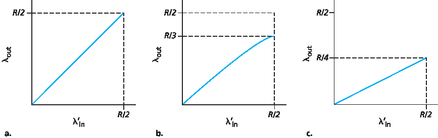
图 3.46 场景2 有限缓冲区下的性能
最后,考虑发送方可能因超时过早而重传尚未丢失但在队列中延迟的分组。此时,原始数据包和重传包可能都到达接收端。接收端只需一份拷贝,会丢弃重传包。此时路由器转发重传包所做的工作是浪费,因为接收端已收到原始包。路由器本可用这部分链路容量传送其他分组。这里又是拥塞网络的另一代价——发送方因较大延迟导致的无谓重传使路由器使用链路带宽转发不必要的分组副本。图3.46(c) 显示在假设路由器平均转发每个分组两次时,吞吐量随负载输入变化的关系。由于每个分组被转发两次,负载输入逼近 R/2 时,吞吐量的渐近值为 R/4。
Let’s now slightly modify scenario 1 in the following two ways (see Figure 3.45). First, the amount of router buffering is assumed to be finite. A consequence of this real-world assumption is that packets will be dropped when arriving to an already-full buffer. Second, we assume that each connection is reliable. If a packet containing a transport-level segment is dropped at the router, the sender will eventually retransmit it. Because packets can be retransmitted, we must now be more careful with our use of the term sending rate. Specifically, let us again denote the rate at which the application sends original data into the socket by λin bytes/sec. The rate at which the transport layer sends segments (containing original data and retransmitted data) into the network will be denoted λ‘in bytes/sec. λ’in is sometimes referred to as the offered load to the network.
Figure 3.45 Scenario 2: Two hosts (with retransmissions) and a router with finite buffers
The performance realized under scenario 2 will now depend strongly on how retransmission is performed. First, consider the unrealistic case that Host A is able to somehow (magically!) determine whether or not a buffer is free in the router and thus sends a packet only when a buffer is free. In this case, no loss would occur, λin would be equal to λ′in, and the throughput of the connection would be equal to λin. This case is shown in Figure 3.46(a). From a throughput standpoint, performance is ideal—everything that is sent is received. Note that the average host sending rate cannot exceed R/2 under this scenario, since packet loss is assumed never to occur.
Consider next the slightly more realistic case that the sender retransmits only when a packet is known for certain to be lost. (Again, this assumption is a bit of a stretch. However, it is possible that the sending host might set its timeout large enough to be virtually assured that a packet that has not been acknowledged has been lost.) In this case, the performance might look something like that shown in Figure 3.46(b). To appreciate what is happening here, consider the case that the offered load, λ′in (the rate of original data transmission plus retransmissions), equals R/2. According to Figure 3.46(b), at this value of the offered load, the rate at which data are delivered to the receiver application is R/3. Thus, out of the 0.5R units of data transmitted, 0.333R bytes/sec (on average) are original data and 0.166R bytes/sec (on average) are retransmitted data. We see here another cost of a congested network—the sender must perform retransmissions in order to compensate for dropped (lost) packets due to buffer overflow.
Figure 3.46 Scenario 2 performance with finite buffers
Finally, let us consider the case that the sender may time out prematurely and retransmit a packet that has been delayed in the queue but not yet lost. In this case, both the original data packet and the retransmission may reach the receiver. Of course, the receiver needs but one copy of this packet and will discard the retransmission. In this case, the work done by the router in forwarding the retransmitted copy of the original packet was wasted, as the receiver will have already received the original copy of this packet. The router would have better used the link transmission capacity to send a different packet instead. Here then is yet another cost of a congested network—unneeded retransmissions by the sender in the face of large delays may cause a router to use its link bandwidth to forward unneeded copies of a packet. Figure 3.46 (c) shows the throughput versus offered load when each packet is assumed to be forwarded (on average) twice by the router. Since each packet is forwarded twice, the throughput will have an asymptotic value of R/4 as the offered load approaches R/2.
场景3:四个发送方,具有有限缓冲区的路由器,以及多跳路径#
Scenario 3: Four Senders, Routers with Finite Buffers, and Multihop Paths
在我们最后的拥塞场景中,四个主机通过相互重叠的两跳路径发送分组,如 图3.47 所示。我们再次假设每个主机都使用超时/重传机制来实现可靠的数据传输服务,所有主机具有相同的 λin 值,且所有路由器链路的容量均为 R 字节/秒。
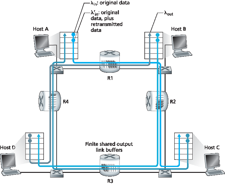
图 3.47 四个发送方,具有有限缓冲区的路由器和多跳路径
考虑主机 A 到主机 C 的连接,该连接经过路由器 R1 和 R2。A–C 连接与 D–B 连接共享路由器 R1,与 B–D 连接共享路由器 R2。对于极小的 \(λ_{in}\) 值,缓冲区溢出较少(如拥塞场景1和2),吞吐量大致等于负载输入。对于稍大一点的 \(λ_{in}\),相应的吞吐量也更大,因为更多的原始数据被发送到网络并传送到目的地,且溢出仍然罕见。因此,对于小的 \(λ_{in}\),增加 \(λ_{in}\) 会导致 \(λ_{out}\) 增加。
考虑极低流量情况后,我们接下来考察 λin(因此 λ’in)极大的情况。考虑路由器 R2。流经 R1 并转发到 R2 的 A–C 流量在 R2 的到达速率最多为 R,即从 R1 到 R2 链路的容量,无论 \(λ_{in}\) 的值是多少。如果所有连接(包括 B–D 连接)的 λ‘in 极大,则 B–D 流量在 R2 的到达速率可以远大于 A–C 流量。由于 A–C 和 B–D 流量必须在路由器 R2 竞争有限的缓冲空间,随着 B–D 的负载输入越来越大,成功通过 R2 的 A–C 流量(即未因缓冲溢出丢失的流量)变得越来越少。极限情况下,当负载输入趋近于无穷大时,R2 的空缓冲区将立即被 B–D 分组填满,A–C 连接在 R2 的吞吐量趋近于零。这反过来意味着,在极高流量极限下,A–C 的端到端吞吐量也趋近于零。上述考虑导致了 图3.48 所示的负载输入与吞吐量之间的权衡关系。
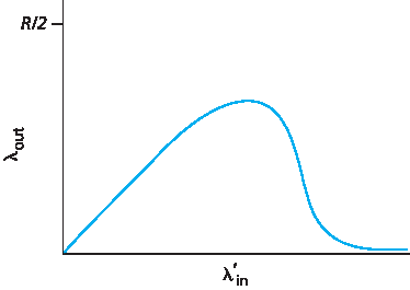
图 3.48 场景3 有限缓冲区和多跳路径下的性能
吞吐量随负载输入增加而最终下降的原因,在于网络所做的无效工作量。上述高流量场景中,每当一个分组在第二跳路由器被丢弃,第一跳路由器转发该分组所做的工作即被“浪费”。如果第一跳路由器直接丢弃该分组并保持空闲,网络状态也将同样糟糕(更准确地说,效果一样差)。更重要的是,第一跳路由器用于转发分组到第二跳的传输容量,本可更有效地用于发送其他分组。(例如,路由器在选择分组进行传输时,可能更应该优先转发已经过若干上游路由器的分组。)因此,这里又体现了因拥塞丢包的另一代价——当路径上的分组被丢弃时,分组从源头到丢弃点的所有上游链路传输容量均被浪费了。
In our final congestion scenario, four hosts transmit packets, each over overlapping two-hop paths, as shown in Figure 3.47. We again assume that each host uses a timeout/retransmission mechanism to implement a reliable data transfer service, that all hosts have the same value of λin, and that all router links have capacity R bytes/sec.
Figure 3.47 Four senders, routers with finite buffers, and multihop paths
Let’s consider the connection from Host A to Host C, passing through routers R1 and R2. The A–C connection shares router R1 with the D–B connection and shares router R2 with the B–D connection. For extremely small values of \(λ_{in}\), buffer overflows are rare (as in congestion scenarios 1 and 2), and the throughput approximately equals the offered load. For slightly larger values of \(λ_{in}\), the corresponding throughput is also larger, since more original data is being transmitted into the network and delivered to the destination, and overflows are still rare. Thus, for small values of \(λ_{in}\), an increase in \(λ_{in}\) results in an increase in \(λ_{out}\).
Having considered the case of extremely low traffic, let’s next examine the case that λin (and hence λ’in) is extremely large. Consider router R2. The A–C traffic arriving to router R2 (which arrives at R2 after being forwarded from R1) can have an arrival rate at R2 that is at most R, the capacity of the link from R1 to R2, regardless of the value of \(λ_{in}\). If λ′in is extremely large for all connections (including the B–D connection), then the arrival rate of B–D traffic at R2 can be much larger than that of the A–C traffic. Because the A–C and B–D traffic must compete at router R2 for the limited amount of buffer space, the amount of A–C traffic that successfully gets through R2 (that is, is not lost due to buffer overflow) becomes smaller and smaller as the offered load from B–D gets larger and larger. In the limit, as the offered load approaches infinity, an empty buffer at R2 is immediately filled by a B–D packet, and the throughput of the A–C connection at R2 goes to zero. This, in turn, implies that the A–C end-to-end throughput goes to zero in the limit of heavy traffic. These considerations give rise to the offered load versus throughput tradeoff shown in Figure 3.48.
Figure 3.48 Scenario 3 performance with finite buffers and multihop paths
The reason for the eventual decrease in throughput with increasing offered load is evident when one considers the amount of wasted work done by the network. In the high-traffic scenario outlined above, whenever a packet is dropped at a second-hop router, the work done by the first-hop router in forwarding a packet to the second-hop router ends up being “wasted.” The network would have been equally well off (more accurately, equally bad off) if the first router had simply discarded that packet and remained idle. More to the point, the transmission capacity used at the first router to forward the packet to the second router could have been much more profitably used to transmit a different packet. (For example, when selecting a packet for transmission, it might be better for a router to give priority to packets that have already traversed some number of upstream routers.) So here we see yet another cost of dropping a packet due to congestion—when a packet is dropped along a path, the transmission capacity that was used at each of the upstream links to forward that packet to the point at which it is dropped ends up having been wasted.
3.6.2 拥塞控制方法#
3.6.2 Approaches to Congestion Control
在 第3.7节 中,我们将详细探讨 TCP 具体的拥塞控制方法。这里,我们先介绍实践中采取的两大类拥塞控制方法,并讨论体现这些方法的具体网络架构和拥塞控制协议。
在最高层次上,我们可以根据网络层是否为传输层提供明确的拥塞控制支持,将拥塞控制方法区分为:
端到端拥塞控制。端到端拥塞控制方法中,网络层不为传输层提供明确的拥塞控制支持。即使网络拥塞的存在,也必须由端系统仅基于观察到的网络行为(如分组丢失和延迟)推断出来。我们将在 第3.7.1节 中看到,TCP 采用这种端到端方法进行拥塞控制,因为 IP 层不需要向主机反馈网络拥塞信息。TCP 分组丢失(由超时或收到三个重复确认标识)被视为网络拥塞的标志,TCP 相应减少窗口大小。我们还将看到一种较新的 TCP 拥塞控制提议,它使用往返时延增加作为网络拥塞加剧的指标。
网络辅助拥塞控制。网络辅助拥塞控制中,路由器向发送方和/或接收方提供关于网络拥塞状态的明确反馈。这种反馈可能非常简单,例如单个位指示链路拥塞——这是早期 IBM SNA [Schwartz 1982]、DEC DECnet [ Jain 1989;Ramakrishnan 1990] 架构和 ATM [Black 1995] 网络架构采取的方法。也可提供更复杂的反馈。例如,在 ATM 可用比特率(ABR) 拥塞控制中,路由器向发送方告知其可支持的最大主机发送速率。如上所述,互联网默认的 IP 和 TCP 版本采用端到端拥塞控制方法。但我们将在 第3.7.2节 看到,近年来 IP 和 TCP 也可选择性地实现网络辅助拥塞控制。
对于网络辅助拥塞控制,拥塞信息通常通过以下两种方式之一从网络反馈给发送方,如 图3.49 所示。第一种是路由器直接向发送方发送反馈。这种通知通常以“拥塞包”(choke packet)的形式出现(本质上表示“我这里拥塞了!”)。第二种更常见的通知方式是,路由器在从发送方到接收方的数据包中标记或更新字段以指示拥塞。接收方收到带标记的分组后,再通知发送方拥塞信息。后一种通知方式需要一个完整的往返时间。
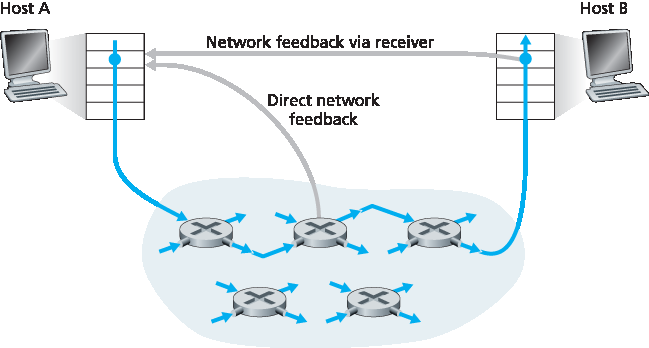
图 3.49 网络指示的拥塞信息的两种反馈路径
In Section 3.7, we’ll examine TCP’s specific approach to congestion control in great detail. Here, we identify the two broad approaches to congestion control that are taken in practice and discuss specific network architectures and congestion-control protocols embodying these approaches.
At the highest level, we can distinguish among congestion-control approaches by whether the network layer provides explicit assistance to the transport layer for congestion-control purposes:
End-to-end congestion control. In an end-to-end approach to congestion control, the network layer provides no explicit support to the transport layer for congestion-control purposes. Even the presence of network congestion must be inferred by the end systems based only on observed network behavior (for example, packet loss and delay). We’ll see shortly in Section 3.7.1 that TCP takes this end-to-end approach toward congestion control, since the IP layer is not required to provide feedback to hosts regarding network congestion. TCP segment loss (as indicated by a timeout or the receipt of three duplicate acknowledgments) is taken as an indication of network congestion, and TCP decreases its window size accordingly. We’ll also see a more recent proposal for TCP congestion control that uses increasing round-trip segment delay as an indicator of increased network congestion
Network-assisted congestion control. With network-assisted congestion control, routers provide explicit feedback to the sender and/or receiver regarding the congestion state of the network. This feedback may be as simple as a single bit indicating congestion at a link – an approach taken in the early IBM SNA [Schwartz 1982], DEC DECnet [ Jain 1989 ; Ramakrishnan 1990] architectures, and ATM [Black 1995] network architectures. More sophisticated feedback is also possible. For example, in ATM Available Bite Rate (ABR) congestion control, a router informs the sender of the maximum host sending rate it (the router) can support on an outgoing link. As noted above, the Internet-default versions of IP and TCP adopt an end-to-end approach towards congestion control. We’ll see, however, in Section 3.7.2 that, more recently, IP and TCP may also optionally implement network-assisted congestion control.
For network-assisted congestion control, congestion information is typically fed back from the network to the sender in one of two ways, as shown in Figure 3.49. Direct feedback may be sent from a network router to the sender. This form of notification typically takes the form of a choke packet (essentially saying, “I’m congested!”). The second and more common form of notification occurs when a router marks/updates a field in a packet flowing from sender to receiver to indicate congestion. Upon receipt of a marked packet, the receiver then notifies the sender of the congestion indication. This latter form of notification takes a full round-trip time.
Figure 3.49 Two feedback pathways for network-indicated congestion information