9.3 基于 IP 的语音通信#
9.3 Voice-over-IP
互联网上的实时对话语音常被称为 网络电话(Internet telephony),因为从用户的角度来看,它类似于传统的电路交换电话服务。它也通常被称为 VoIP(Voice-over-IP)。在本节中,我们将介绍 VoIP 的原理和协议。会话视频在许多方面与 VoIP 类似,不同之处在于它包含了参与者的视频画面以及语音。为了使讨论更集中和具体,本节仅关注语音,而非语音与视频的组合。
Real-time conversational voice over the Internet is often referred to as Internet telephony, since, from the user’s perspective, it is similar to the traditional circuit-switched telephone service. It is also commonly called Voice-over-IP (VoIP). In this section we describe the principles and protocols underlying VoIP. Conversational video is similar in many respects to VoIP, except that it includes the video of the participants as well as their voices. To keep the discussion focused and concrete, we focus here only on voice in this section rather than combined voice and video.
9.3.1 尽力而为(Best-Effort)IP 服务的局限性#
9.3.1 Limitations of the Best-Effort IP Service
互联网的网络层协议 IP 提供的是尽力而为服务。也就是说,该服务尽最大努力将每个数据报从源头传输到目的地,但不对数据包在某个延迟范围内成功到达目的地作出任何承诺,也不保证丢包率在某一限制之内。这种缺乏保障的服务对实时会话类应用(如 VoIP)设计带来了重大挑战,因为这些应用对数据包的延迟、抖动和丢失极为敏感。
在本节中,我们将介绍几种在尽力而为网络上提升 VoIP 性能的方法。我们将重点讨论应用层技术,也就是说,这些方法不需要更改网络核心,甚至不需要更改终端系统中的传输层。为了使讨论更具实效性,我们将在一个具体的 VoIP 示例中讨论尽力而为 IP 服务的局限性。发送方以 8,000 字节/秒的速率生成字节;每隔 20 毫秒,发送方将这些字节收集成一个数据块。该数据块和一个特殊的头部(稍后讨论)被封装到一个 UDP 段中,并通过套接字接口发送。因此,每个数据块的字节数为 (20 毫秒)⋅(8,000 字节/秒)=160 字节,每 20 毫秒发送一个 UDP 段。
如果每个数据包都以恒定的端到端延迟到达接收端,那么接收端每隔 20 毫秒就会周期性地接收到一个数据包。在这种理想情况下,接收端只需在数据块到达时立即播放即可。但不幸的是,即使在轻度拥塞的网络中,也会有部分数据包丢失,而且大多数数据包的端到端延迟也不相同。因此,接收端必须更加谨慎地决定 (1) 何时播放数据块,(2) 如何处理缺失的数据块。
The Internet’s network-layer protocol, IP, provides best-effort service. That is to say the service makes its best effort to move each datagram from source to destination as quickly as possible but makes no promises whatsoever about getting the packet to the destination within some delay bound or about a limit on the percentage of packets lost. The lack of such guarantees poses significant challenges to the design of real-time conversational applications, which are acutely sensitive to packet delay, jitter, and loss.
In this section, we’ll cover several ways in which the performance of VoIP over a best-effort network can be enhanced. Our focus will be on application-layer techniques, that is, approaches that do not require any changes in the network core or even in the transport layer at the end hosts. To keep the discussion concrete, we’ll discuss the limitations of best-effort IP service in the context of a specific VoIP example. The sender generates bytes at a rate of 8,000 bytes per second; every 20 msecs the sender gathers these bytes into a chunk. A chunk and a special header (discussed below) are encapsulated in a UDP segment, via a call to the socket interface. Thus, the number of bytes in a chunk is (20 msecs)⋅(8,000 bytes/sec)=160 bytes, and a UDP segment is sent every 20 msecs.
If each packet makes it to the receiver with a constant end-to-end delay, then packets arrive at the receiver periodically every 20 msecs. In these ideal conditions, the receiver can simply play back each chunk as soon as it arrives. But unfortunately, some packets can be lost and most packets will not have the same end-to-end delay, even in a lightly congested Internet. For this reason, the receiver must take more care in determining (1) when to play back a chunk, and (2) what to do with a missing chunk.
数据包丢失#
Packet Loss
考虑我们的 VoIP 应用生成的一个 UDP 段。该 UDP 段被封装在一个 IP 数据报中。当数据报在网络中传输时,会穿越多个路由器缓冲区(即队列),在出接口等待发送。如果从发送方到接收方的路径上的某个或多个缓冲区已满,则到达的数据报可能会被丢弃,永远无法到达接收端应用程序。
如果使用 TCP(它提供可靠数据传输)而不是 UDP 来发送数据包,就可以消除丢包现象。然而,对于像 VoIP 这样的实时音频会话应用来说,重传机制通常被认为是不可接受的,因为它会增加端到端延迟 [Bolot 1996]。此外,由于 TCP 拥塞控制机制,数据包丢失可能导致 TCP 发送方的传输速率下降到低于接收方读取速率,从而可能导致缓冲区耗尽。这会严重影响接收端的语音清晰度。因此,大多数现有的 VoIP 应用默认运行在 UDP 之上。[Baset 2006] 报道称,除非用户处于阻止 UDP 段的 NAT 或防火墙之后,否则 Skype 使用 UDP。
但数据包丢失并不一定如人们想象的那样灾难性。实际上,丢包率在 1% 到 20% 之间是可以容忍的,这取决于语音的编码和传输方式,以及接收端如何掩盖丢包。例如,前向纠错(FEC)可以帮助掩盖丢失的数据包。我们将在下文看到,使用 FEC 时,冗余信息与原始信息一起传输,从而可以从冗余信息中恢复部分丢失的原始数据。然而,如果发送方与接收方之间的一个或多个链路严重拥塞,导致丢包率超过 10% 到 20%(例如在无线链路上),那么几乎无法获得可接受的音频质量。显然,尽力而为服务是有局限性的。
Consider one of the UDP segments generated by our VoIP application. The UDP segment is encapsulated in an IP datagram. As the datagram wanders through the network, it passes through router buffers (that is, queues) while waiting for transmission on outbound links. It is possible that one or more of the buffers in the path from sender to receiver is full, in which case the arriving IP datagram may be discarded, never to arrive at the receiving application.
Loss could be eliminated by sending the packets over TCP (which provides for reliable data transfer) rather than over UDP. However, retransmission mechanisms are often considered unacceptable for conversational real-time audio applications such as VoIP, because they increase end-to-end delay [Bolot 1996]. Furthermore, due to TCP congestion control, packet loss may result in a reduction of the TCP sender’s transmission rate to a rate that is lower than the receiver’s drain rate, possibly leading to buffer starvation. This can have a severe impact on voice intelligibility at the receiver. For these reasons, most existing VoIP applications run over UDP by default. [Baset 2006] reports that UDP is used by Skype unless a user is behind a NAT or firewall that blocks UDP segments (in which case TCP is used).
But losing packets is not necessarily as disastrous as one might think. Indeed, packet loss rates between 1 and 20 percent can be tolerated, depending on how voice is encoded and transmitted, and on how the loss is concealed at the receiver. For example, forward error correction (FEC) can help conceal packet loss. We’ll see below that with FEC, redundant information is transmitted along with the original information so that some of the lost original data can be recovered from the redundant information. Nevertheless, if one or more of the links between sender and receiver is severely congested, and packet loss exceeds 10 to 20 percent (for example, on a wireless link), then there is really nothing that can be done to achieve acceptable audio quality. Clearly, best-effort service has its limitations.
端到端延迟#
End-to-End Delay
端到端延迟 是指路由器中的传输、处理和排队延迟;链路中的传播延迟;以及端系统的处理延迟的总和。对于像 VoIP 这样的实时会话类应用,端到端延迟小于 150 毫秒对人类听众是不可察觉的;150 到 400 毫秒之间的延迟可以接受,但并不理想;而超过 400 毫秒的延迟则会严重影响语音会话的交互性。VoIP 应用的接收端通常会忽略超过某一阈值的延迟数据包,例如超过 400 毫秒的延迟。因此,延迟超过阈值的数据包实际上也被视为丢失。
End-to-end delay is the accumulation of transmission, processing, and queuing delays in routers; propagation delays in links; and end-system processing delays. For real-time conversational applications, such as VoIP, end-to-end delays smaller than 150 msecs are not perceived by a human listener; delays between 150 and 400 msecs can be acceptable but are not ideal; and delays exceeding 400 msecs can seriously hinder the interactivity in voice conversations. The receiving side of a VoIP application will typically disregard any packets that are delayed more than a certain threshold, for example, more than 400 msecs. Thus, packets that are delayed by more than the threshold are effectively lost.
数据包抖动#
Packet Jitter
端到端延迟的一个关键组成部分是数据包在网络路由器中所经历的排队延迟的变化。由于这些变化,每个数据包从源端生成到接收端接收的时间可能会有所不同,如 Figure 9.1 所示。这种现象称为 抖动(jitter)。例如,考虑 VoIP 应用中两个连续的数据包。发送方在发送第一个数据包后 20 毫秒发送第二个数据包。但在接收方,这两个数据包的间隔可能大于 20 毫秒。要理解这一点,假设第一个数据包到达路由器时排队很短,而在第二个数据包到达前,大量来自其他源的数据包也到达了该队列。由于第一个数据包经历了较小的排队延迟,而第二个数据包经历了较大的排队延迟,这两个数据包在接收端的时间间隔就超过了 20 毫秒。
相反,两个连续数据包的间隔也可能小于 20 毫秒。例如,假设第一个数据包排在一个较长队列的末尾,而第二个数据包在第一个数据包发送之前就到达了队列,并且在此之前没有来自其他源的数据包。在这种情况下,这两个数据包将紧挨着排在队列中。如果路由器出接口发送一个数据包所需的时间小于 20 毫秒,那么两个数据包的间隔也将小于 20 毫秒。
这种情况类似于汽车在道路上行驶。假设你和你的朋友分别驾驶自己的汽车从圣地亚哥前往凤凰城。你们的驾驶风格相似,在交通允许的情况下都以 100 公里/小时的速度行驶。如果你的朋友比你早一个小时出发,那么根据途中交通状况,你到达凤凰城的时间可能比你朋友早也可能比他晚。
如果接收方忽略抖动的存在,并在数据块到达时立即播放,那么接收方所听到的音频质量可能会变得难以理解。幸运的是,通常可以使用 序列号、 时间戳 和 播放延迟(playout delay) 来消除抖动,这将在下文中讨论。
A crucial component of end-to-end delay is the varying queuing delays that a packet experiences in the network’s routers. Because of these varying delays, the time from when a packet is generated at the source until it is received at the receiver can fluctuate from packet to packet, as shown in Figure 9.1. This phenomenon is called jitter. As an example, consider two consecutive packets in our VoIP application. The sender sends the second packet 20 msecs after sending the first packet. But at the receiver, the spacing between these packets can become greater than 20 msecs. To see this, suppose the first packet arrives at a nearly empty queue at a router, but just before the second packet arrives at the queue a large number of packets from other sources arrive at the same queue. Because the first packet experiences a small queuing delay and the second packet suffers a large queuing delay at this router, the first and second packets become spaced by more than 20 msecs. The spacing between consecutive packets can also become less than 20 msecs. To see this, again consider two consecutive packets. Suppose the first packet joins the end of a queue with a large number of packets, and the second packet arrives at the queue before this first packet is transmitted and before any packets from other sources arrive at the queue. In this case, our two packets find themselves one right after the other in the queue. If the time it takes to transmit a packet on the router’s outbound link is less than 20 msecs, then the spacing between first and second packets becomes less than 20 msecs.
The situation is analogous to driving cars on roads. Suppose you and your friend are each driving in your own cars from San Diego to Phoenix. Suppose you and your friend have similar driving styles, and that you both drive at 100 km/hour, traffic permitting. If your friend starts out one hour before you, depending on intervening traffic, you may arrive at Phoenix more or less than one hour after your friend.
If the receiver ignores the presence of jitter and plays out chunks as soon as they arrive, then the resulting audio quality can easily become unintelligible at the receiver. Fortunately, jitter can often be removed by using sequence numbers, timestamps, and a playout delay, as discussed below.
9.3.2 接收端消除音频抖动#
9.3.2 Removing Jitter at the Receiver for Audio
对于我们的 VoIP 应用,数据包是周期性生成的,接收端应尝试在存在随机网络抖动的情况下,周期性地播放语音数据块。通常通过结合以下两种机制实现:
在每个数据块前加上时间戳。发送端为每个数据块打上生成时间的时间戳。
接收端延迟播放数据块。如我们在前面对 图 9.1 的讨论所示,接收的音频数据块的播放延迟必须足够长,以确保大多数数据包在其预定的播放时间之前到达。这个播放延迟可以在整个音频会话期间保持固定,也可以在会话期间自适应变化。
下面我们讨论这三种机制结合起来如何缓解甚至消除抖动的影响。我们考察两种播放策略:固定播放延迟和自适应播放延迟。
For our VoIP application, where packets are being generated periodically, the receiver should attempt to provide periodic playout of voice chunks in the presence of random network jitter. This is typically done by combining the following two mechanisms:
Prepending each chunk with a timestamp. The sender stamps each chunk with the time at which the chunk was generated.
Delaying playout of chunks at the receiver. As we saw in our earlier discussion of Figure 9.1, the playout delay of the received audio chunks must be long enough so that most of the packets are received before their scheduled playout times. This playout delay can either be fixed throughout the duration of the audio session or vary adaptively during the audio session lifetime.
We now discuss how these three mechanisms, when combined, can alleviate or even eliminate the effects of jitter. We examine two playback strategies: fixed playout delay and adaptive playout delay.
固定播放延迟#
Fixed Playout Delay
采用固定延迟策略时,接收端试图在数据块生成后恰好 q 毫秒时播放该数据块。因此,如果数据块在发送端被打上时间戳 t,接收端将在 t+q 时播放该数据块,前提是数据块已在此之前到达。超过预定播放时间到达的数据包将被丢弃,视为丢失。
那么 q 应该如何选择?VoIP 可以支持最高约 400 毫秒的延迟,尽管较小的 q 会带来更满意的对话体验。另一方面,如果 q 远小于 400 毫秒,则由于网络引起的抖动,许多数据包可能会错过其预定播放时间。大体来说,如果端到端延迟变化较大,倾向于使用较大的 q;如果延迟较小且变化也小,则倾向于使用较小的 q,可能小于 150 毫秒。
图 9.4 展示了播放延迟与丢包率之间的权衡。图中显示了单次讲话段中数据包的生成和播放时间,考虑了两个不同的初始播放延迟。如最左侧阶梯状曲线所示,发送方以固定间隔生成数据包——比如每 20 毫秒。该讲话段的第一个数据包在时间 r 被接收。图中显示,后续数据包的到达间隔由于网络抖动而不均匀。
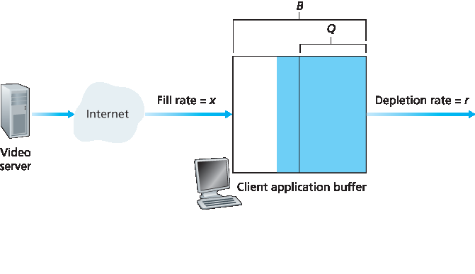
图 9.4 不同固定播放延迟下的数据包丢失
对于第一个播放时间表,固定的初始播放延迟设为 p−r。在此时间表下,第四个数据包未能按时到达,接收端视其为丢失。对于第二个播放时间表,固定的初始播放延迟设为 p′−r。此时间表下,所有数据包均在预定播放时间之前到达,因此无丢包。
With the fixed-delay strategy, the receiver attempts to play out each chunk exactly q msecs after the chunk is generated. So if a chunk is timestamped at the sender at time t, the receiver plays out the chunk at time t+q, assuming the chunk has arrived by that time. Packets that arrive after their scheduled playout times are discarded and considered lost.
What is a good choice for q? VoIP can support delays up to about 400 msecs, although a more satisfying conversational experience is achieved with smaller values of q. On the other hand, if q is made much smaller than 400 msecs, then many packets may miss their scheduled playback times due to the network-induced packet jitter. Roughly speaking, if large variations in end-to-end delay are typical, it is preferable to use a large q; on the other hand, if delay is small and variations in delay are also small, it is preferable to use a small q, perhaps less than 150 msecs.
The trade-off between the playback delay and packet loss is illustrated in Figure 9.4. The figure shows the times at which packets are generated and played out for a single talk spurt. Two distinct initial playout delays are considered. As shown by the leftmost staircase, the sender generates packets at regular intervals—say, every 20 msecs. The first packet in this talk spurt is received at time r. As shown in the figure, the arrivals of subsequent packets are not evenly spaced due to the network jitter.
Figure 9.4 Packet loss for different fixed playout delays
For the first playout schedule, the fixed initial playout delay is set to p−r. With this schedule, the fourth packet does not arrive by its scheduled playout time, and the receiver considers it lost. For the second playout schedule, the fixed initial playout delay is set to p′−r. For this schedule, all packets arrive before their scheduled playout times, and there is therefore no loss.
自适应播放延迟#
Adaptive Playout Delay
前例展示了设计固定播放延迟策略时出现的重要延迟与丢包权衡。通过增大初始播放延迟,大多数数据包可按时到达,丢包率几乎为零;然而,对于像 VoIP 这样的对话服务,过长的延迟会令人不适甚至无法容忍。理想情况下,我们希望在丢包率低于几个百分点的前提下,将播放延迟降到最低。
解决这一权衡的自然方法是估计网络延迟及其方差,并在每个讲话段开始时相应调整播放延迟。讲话段开始时对播放延迟的自适应调整会导致发送方的静默期被压缩或延长;不过,少量的静默期压缩或延长在人声中不易被察觉。
参照 [Ramjee 1994],我们现描述接收端可用于自适应调整播放延迟的通用算法。设
ti= 第 i 个数据包的时间戳 = 发送端生成该数据包的时间
ri= 第 i 个数据包被接收端接收的时间
pi= 第 i 个数据包在接收端的播放时间
第 i 个数据包的端到端网络延迟为 ri−ti。由于网络抖动,该延迟会在数据包间波动。令 di 表示接收第 i 个数据包时的网络平均延迟估计。该估计由时间戳计算得出:
di=(1−u)di−1+u(ri−ti)
其中 u 是固定常数(例如 u=0.01)。因此 di 是观测到的网络延迟 r1−t1,…,ri−ti 的平滑平均值。该估计对最近观测的网络延迟赋予更大权重,对较早的延迟赋予较小权重。这种估计形式并不陌生;类似的方法用于估计 TCP 的往返时延,如 第3章 所述。令 vi 表示网络延迟相对于平均延迟的平均偏差估计。该估计同样由时间戳计算:
vi=(1−u)vi−1+u| ri−ti−di|
对每个接收的数据包计算估计值 di 和 vi,但它们仅用于确定任何讲话段中第一个数据包的播放点。
计算出这些估计后,接收端采用如下算法播放数据包。若数据包 i 是讲话段的第一个包,则其播放时间 pi 计算为:
pi=ti+di+Kvi
其中 K 是正常数(例如 K=4)。Kvi 项的作用是将播放时间设置得足够靠后,使得只有极少数讲话段中的数据包因迟到而丢失。讲话段中随后的任意数据包的播放点相对于讲话段第一个包的播放时间偏移量计算。具体地,设
qi=pi−ti
为讲话段第一个包从生成到播放的时间间隔。若数据包 j 属于该讲话段,则播放时间为
pj=tj+qi
该算法在假设接收端能识别讲话段第一个包的情况下完全合理。接收端可通过检测每个接收包的信号能量实现此识别。
The previous example demonstrates an important delay-loss trade-off that arises when designing a playout strategy with fixed playout delays. By making the initial playout delay large, most packets will make their deadlines and there will therefore be negligible loss; however, for conversational services such as VoIP, long delays can become bothersome if not intolerable. Ideally, we would like the playout delay to be minimized subject to the constraint that the loss be below a few percent.
The natural way to deal with this trade-off is to estimate the network delay and the variance of the network delay, and to adjust the playout delay accordingly at the beginning of each talk spurt. This adaptive adjustment of playout delays at the beginning of the talk spurts will cause the sender’s silent periods to be compressed and elongated; however, compression and elongation of silence by a small amount is not noticeable in speech.
Following [Ramjee 1994], we now describe a generic algorithm that the receiver can use to adaptively adjust its playout delays. To this end, let
ti= the timestamp of the ith packet = the time the packet was generated by the sender
ri= the time packet i is received by receiver
pi= the time packet i is played at receiver
The end-to-end network delay of the ith packet is ri−ti. Due to network jitter, this delay will vary from packet to packet. Let di denote an estimate of the average network delay upon reception of the ith packet. This estimate is constructed from the timestamps as follows:
di=(1−u)di−1+u(ri−ti)
where u is a fixed constant (for example, u=0.01). Thus di is a smoothed average of the observed network delays r1−t1,…,ri−ti. The estimate places more weight on the recently observed network delays than on the observed network delays of the distant past. This form of estimate should not be completely unfamiliar; a similar idea is used to estimate round-trip times in TCP, as discussed in Chapter 3. Let vi denote an estimate of the average deviation of the delay from the estimated average delay. This estimate is also constructed from the timestamps:
vi=(1−u)vi−1+u| ri−ti−di|
The estimates di and vi are calculated for every packet received, although they are used only to determine the playout point for the first packet in any talk spurt.
Once having calculated these estimates, the receiver employs the following algorithm for the playout of packets. If packet i is the first packet of a talk spurt, its playout time, pi, is computed as:
pi=ti+di+Kvi
where K is a positive constant (for example, K=4). The purpose of the Kvi term is to set the playout time far enough into the future so that only a small fraction of the arriving packets in the talk spurt will be lost due to late arrivals. The playout point for any subsequent packet in a talk spurt is computed as an offset from the point in time when the first packet in the talk spurt was played out. In particular, let
qi=pi−ti
be the length of time from when the first packet in the talk spurt is generated until it is played out. If packet j also belongs to this talk spurt, it is played out at time
pj=tj+qi
The algorithm just described makes perfect sense assuming that the receiver can tell whether a packet is the first packet in the talk spurt. This can be done by examining the signal energy in each received packet.
9.3.3 从数据包丢失中恢复#
9.3.3 Recovering from Packet Loss
我们已经详细讨论了 VoIP 应用如何应对数据包抖动。现在简要介绍几种在数据包丢失情况下努力保持可接受音频质量的方案。这些方案称为 丢包恢复方案。这里我们对数据包丢失的定义较宽泛:数据包如果从未到达接收端,或者到达时间晚于预定播放时间,则视为丢失。我们将再次以 VoIP 例子作为描述丢包恢复方案的背景。
正如本节开头提到的,实时对话应用如 VoIP 中,重传丢失的数据包往往不可行。实际上,重传错过播放截止时间的数据包毫无意义。且由于路由器队列溢出导致的数据包丢失,通常无法快速完成重传。基于这些考虑,VoIP 应用通常采用某种丢包预防方案。两种丢包预防方案是 前向纠错(FEC) 和 交织(Interleaving)。
We have discussed in some detail how a VoIP application can deal with packet jitter. We now briefly describe several schemes that attempt to preserve acceptable audio quality in the presence of packet loss. Such schemes are called loss recovery schemes. Here we define packet loss in a broad sense: A packet is lost either if it never arrives at the receiver or if it arrives after its scheduled playout time. Our VoIP example will again serve as a context for describing loss recovery schemes.
As mentioned at the beginning of this section, retransmitting lost packets may not be feasible in a real- time conversational application such as VoIP. Indeed, retransmitting a packet that has missed its playout deadline serves absolutely no purpose. And retransmitting a packet that overflowed a router queue cannot normally be accomplished quickly enough. Because of these considerations, VoIP applications often use some type of loss anticipation scheme. Two types of loss anticipation schemes are forward error correction (FEC) and interleaving.
前向纠错(FEC)#
Forward Error Correction (FEC)
FEC 的基本思想是在原始数据包流中添加冗余信息。以微小增加传输速率为代价,冗余信息可用于重建部分丢失数据包的近似或精确版本。参照 [Bolot 1996] 和 [Perkins 1998],我们概述两种简单的 FEC 机制。第一种机制是在每 n 个数据块后发送一个冗余编码块。该冗余块通过对 n 个原始块进行异或运算得到 [Shacham 1990]。这样,若 n+1 个数据包组中任意一个包丢失,接收端都能完整重建该丢失包。但若丢失两个或更多包,接收端则无法重建。通过保持 n+1 的组大小较小,在丢包率不高时能恢复大量丢包。然而,组大小越小,传输速率相对增加越大。具体来说,传输速率增加约 1/n 倍,例如 n=3 时,速率增加 33%。此外,该简单方案会增加播放延迟,因为接收端必须等待接收完整组数据包后才能开始播放。关于 FEC 在多媒体传输中的实际工作细节见 [RFC 5109]。
第二种 FEC 机制是发送低分辨率音频流作为冗余信息。例如,发送端可能生成一个标准音频流和一个对应的低分辨率低比特率音频流。(标准流可为 64 kbps PCM 编码,低质量流可为 13 kbps GSM 编码。)低比特率流称为冗余流。如 图 9.5 所示,发送端将第 n 个包构造成标准流的第 n 个数据块加上冗余流的第 n−1 个数据块。如此,一旦出现非连续丢包,接收端可通过播放随后包中附带的低比特率编码数据块来掩盖丢包。当然,低比特率块质量低于标准块。但以多数高质量块、偶尔低质量块且无丢块的组合,整体音频质量仍然良好。注意此方案中,接收端只需接收两个包即可开始播放,因而增加的播放延迟较小。此外,若低比特率编码远小于标准编码,则传输速率的边际增加也很小。
为应对连续丢包,可采用简单变体。发送端不仅在第 n 个标准块后附加第 n−1 个低比特率块,还可附加第 n−2 个、第 n−3 个等多个低比特率块。通过附加更多低比特率块,接收端在更严苛的最佳努力网络环境中仍能获得可接受的音质。但额外块也会增加传输带宽和播放延迟。
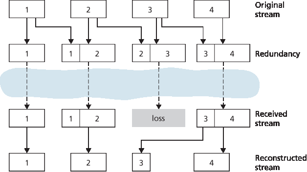
图 9.5 携带低质量冗余信息
The basic idea of FEC is to add redundant information to the original packet stream. For the cost of marginally increasing the transmission rate, the redundant information can be used to reconstruct approximations or exact versions of some of the lost packets. Following [Bolot 1996] and [Perkins 1998], we now outline two simple FEC mechanisms. The first mechanism sends a redundant encoded chunk after every n chunks. The redundant chunk is obtained by exclusive OR-ing the n original chunks [Shacham 1990]. In this manner if any one packet of the group of n+1 packets is lost, the receiver can fully reconstruct the lost packet. But if two or more packets in a group are lost, the receiver cannot reconstruct the lost packets. By keeping n+1, the group size, small, a large fraction of the lost packets can be recovered when loss is not excessive. However, the smaller the group size, the greater the relative increase of the transmission rate. In particular, the transmission rate increases by a factor of 1/n, so that, if n=3, then the transmission rate increases by 33 percent. Furthermore, this simple scheme increases the playout delay, as the receiver must wait to receive the entire group of packets before it can begin playout. For more practical details about how FEC works for multimedia transport see [RFC 5109].
The second FEC mechanism is to send a lower-resolution audio stream as the redundant information. For example, the sender might create a nominal audio stream and a corresponding low-resolution, low- bit rate audio stream. (The nominal stream could be a PCM encoding at 64 kbps, and the lower-quality stream could be a GSM encoding at 13 kbps.) The low-bit rate stream is referred to as the redundant stream. As shown in Figure 9.5, the sender constructs the nth packet by taking the nth chunk from the nominal stream and appending to it the (n−1)st chunk from the redundant stream. In this manner, whenever there is nonconsecutive packet loss, the receiver can conceal the loss by playing out the low- bit rate encoded chunk that arrives with the subsequent packet. Of course, low-bit rate chunks give lower quality than the nominal chunks. However, a stream of mostly high-quality chunks, occasional low- quality chunks, and no missing chunks gives good overall audio quality. Note that in this scheme, the receiver only has to receive two packets before playback, so that the increased playout delay is small. Furthermore, if the low-bit rate encoding is much less than the nominal encoding, then the marginal increase in the transmission rate will be small.
In order to cope with consecutive loss, we can use a simple variation. Instead of appending just the (n−1)st low-bit rate chunk to the nth nominal chunk, the sender can append the (n−1)st and (n−2)nd low- bit rate chunk, or append the (n−1)st and (n−3)rd low-bit rate chunk, and so on. By appending more low- bit rate chunks to each nominal chunk, the audio quality at the receiver becomes acceptable for a wider variety of harsh best-effort environments. On the other hand, the additional chunks increase the transmission bandwidth and the playout delay.
Figure 9.5 Piggybacking lower-quality redundant information
交织#
Interleaving
作为冗余传输的替代方案,VoIP 应用可以发送交织音频。如 图 9.6 所示,发送端在传输前重新排序音频数据单元,使原本相邻的单元在传输流中相隔一定距离。交织能缓解丢包影响。例如,若单元长度为 5 毫秒,数据块为 20 毫秒(即每块包含四个单元),则第一块可能包含单元 1、5、9、13;第二块包含单元 2、6、10、14;依此类推。图 9.6 显示,交织流中单包丢失导致重构流中出现多个小缺口,而非非交织流中的单个大缺口。
交织能显著提升音频流的感知质量 [Perkins 1998],且开销低。明显缺点是增加了延迟,限制了其在 VoIP 等对话应用中的使用,尽管其在存储音频流播放中表现良好。交织的一个主要优点是不会增加流的带宽需求。
As an alternative to redundant transmission, a VoIP application can send interleaved audio. As shown in Figure 9.6, the sender resequences units of audio data before transmission, so that originally adjacent units are separated by a certain distance in the transmitted stream. Interleaving can mitigate the effect of packet losses. If, for example, units are 5 msecs in length and chunks are 20 msecs (that is, four units per chunk), then the first chunk could contain units 1, 5, 9, and 13; the second chunk could contain units 2, 6, 10, and 14; and so on. Figure 9.6 shows that the loss of a single packet from an interleaved stream results in multiple small gaps in the reconstructed stream, as opposed to the single large gap that would occur in a noninterleaved stream.
Interleaving can significantly improve the perceived quality of an audio stream [Perkins 1998]. It also has low overhead. The obvious disadvantage of interleaving is that it increases latency. This limits its use for conversational applications such as VoIP, although it can perform well for streaming stored audio. A major advantage of interleaving is that it does not increase the bandwidth requirements of a stream.
误差掩盖#
Error Concealment
误差掩盖方案试图生成与原包相似的丢包替代品。如 [Perkins 1998] 讨论,由于音频信号,特别是语音,存在大量短期自相似性,此类技术可行。此类技术适用于较低丢包率(低于 15%)和较小包长(4–40 毫秒)。当丢失长度接近音素长度(5–100 毫秒)时,这些技术效果会下降,因为听者可能会错过整个音素。
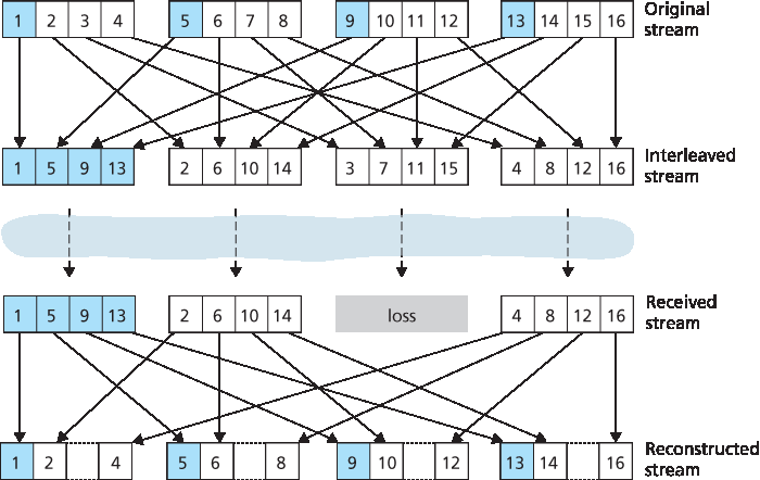
图 9.6 发送交织音频
或许最简单的接收端恢复形式是数据包重复。数据包重复用紧接丢失前的数据包副本替代丢失包,计算复杂度低,表现尚可。另一种接收端恢复是插值,利用丢失前后的音频插值出合适包以覆盖丢失。插值效果优于数据包重复,但计算复杂度显著更高 [Perkins 1998]。
Error concealment schemes attempt to produce a replacement for a lost packet that is similar to the original. As discussed in [Perkins 1998], this is possible since audio signals, and in particular speech, exhibit large amounts of short-term self-similarity. As such, these techniques work for relatively small loss rates (less than 15 percent), and for small packets (4–40 msecs). When the loss length approaches the length of a phoneme (5–100 msecs) these techniques break down, since whole phonemes may be missed by the listener.
Figure 9.6 Sending interleaved audio
Perhaps the simplest form of receiver-based recovery is packet repetition. Packet repetition replaces lost packets with copies of the packets that arrived immediately before the loss. It has low computational complexity and performs reasonably well. Another form of receiver-based recovery is interpolation, which uses audio before and after the loss to interpolate a suitable packet to cover the loss. Interpolation performs somewhat better than packet repetition but is significantly more computationally intensive [Perkins 1998].
9.3.4 案例研究:使用 Skype 的 VoIP#
9.3.4 Case Study: VoIP with Skype
Skype 是一个极为流行的 VoIP 应用,每天有超过 5000 万活跃账户。除了提供主机到主机的 VoIP 服务外,Skype 还提供主机到电话服务、电话到主机服务以及多方主机到主机的视频会议服务。(这里的主机仍指任何连接互联网的 IP 设备,包括个人电脑、平板和智能手机。)Skype 于 2011 年被微软收购。
由于 Skype 协议是专有的,且所有 Skype 的控制包和媒体包均被加密,因此难以精确确定 Skype 的具体工作方式。然而,研究人员通过 Skype 网站和多项测量研究,了解了 Skype 的大致工作原理 [Baset 2006;Guha 2006;Chen 2006;Suh 2006;Ren 2006;Zhang X 2012]。对于语音和视频,Skype 客户端支持多种编解码器,能够以多种码率和质量进行编码。例如,Skype 视频的码率测得最低可达 30 kbps(低质量会话),最高接近 1 Mbps(高质量会话):ref:[Zhang X 2012] <Zhang X 2012>。通常,Skype 的音频质量优于有线电话系统的“普通电话服务”(POTS)质量。(Skype 编解码器通常以 16,000 采样/秒或更高采样率采样语音,提供比 POTS 8,000 采样/秒更丰富的音色。)默认情况下,Skype 通过 UDP 发送音视频包,但控制包通过 TCP 发送,当防火墙阻断 UDP 流时,媒体包也通过 TCP 发送。Skype 对通过 UDP 发送的语音和视频流使用前向纠错(FEC)进行丢包恢复。Skype 客户端还会根据当前网络状况调整发送的音视频流,改变视频质量和 FEC 开销 [Zhang X 2012]。
Skype 在多个创新领域使用 P2P 技术,生动展示了 P2P 可用于超越内容分发和文件共享的应用。与即时通讯类似,主机到主机的互联网电话本质上是 P2P,因为在应用核心,用户对等体(即 peer)实时通信。但 Skype 还将 P2P 用于两个重要功能,即用户定位和 NAT 穿透。
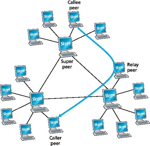
图 9.7 Skype 对等体
如 图 9.7 所示,Skype 中的对等体(主机)被组织成层级覆盖网络,每个对等体被分类为超级节点或普通节点。Skype 维护一个索引,将 Skype 用户名映射到当前 IP 地址(及端口号)。该索引分布于超级节点中。当 Alice 想呼叫 Bob 时,她的 Skype 客户端搜索分布式索引以确定 Bob 当前的 IP 地址。由于 Skype 协议是专有的,目前尚不清楚超级节点间索引映射的具体组织方式,但很可能采用某种 DHT 结构。
Skype 还在 中继 中使用 P2P 技术,这对建立家庭网络中的主机呼叫非常有用。许多家庭网络通过 NAT 访问互联网,如 第 4 章 讨论。回想 NAT 阻止外网主机发起连接到内网主机。如果两个 Skype 用户都处于 NAT 后,问题就出现了——双方都无法接受对方发起的呼叫,导致呼叫看似不可能。超级节点和中继的巧妙使用完美解决了这个问题。假设 Alice 登录时被分配到一个非 NAT 超级节点,并发起与该超级节点的会话。(由于是 Alice 发起,会话被其 NAT 允许。)该会话允许 Alice 与超级节点交换控制消息。Bob 登录时也进行同样操作。现在,当 Alice 想呼叫 Bob 时,她通知自己的超级节点,该超级节点通知 Bob 的超级节点,后者再通知 Bob 有 Alice 的来电。若 Bob 接受呼叫,这两个超级节点会选择第三个非 NAT 超级节点作为中继,其任务是中继 Alice 和 Bob 之间的数据。Alice 和 Bob 的超级节点分别指示两人启动与中继的会话。如 图 9.7 所示,Alice 通过 Alice-中继连接(由 Alice 发起)发送语音包给中继,中继再通过中继-Bob 连接(由 Bob 发起)转发;Bob 到 Alice 的数据包反向通过这两条连接流动。如此,即使双方均无法接受外部发起的会话,仍实现了端到端连接。
至此,我们讨论的 Skype 呼叫仅涉及两人。现在来看多方音频会议。当参与者 N>2 时,若每个用户都将音频流复制发送给其他 N−1 个用户,则总共需要发送 N(N−1) 条音频流到网络中以支持会议。为减少带宽,Skype 采用巧妙的分发技术。具体来说,每个用户将音频流发送给会议发起者,会议发起者将所有音频流合并成一条流(基本上将所有音频信号相加),然后将合并流的副本发送给其他 N−1 个参与者。这样,流数减少为 2(N−1)。对于普通两人视频通话,Skype 采用点对点路由,除非需要 NAT 穿透,则通过非 NAT 节点中继。如前述。对于 N>2 的视频会议,由于视频媒体特性,Skype 不会像语音那样在一个地点合并再分发,而是将每个参与者的视频流路由到一个服务器集群(截至 2011 年位于爱沙尼亚),该集群再将其他 N−1 个参与者的视频流转发给该参与者 [Zhang X 2012]。你可能疑惑为何参与者将视频流发送给服务器,而非直接发送给其他 N−1 个参与者?两种方法都涉及 N(N−1) 条视频流被参与者接收。原因在于,大多数接入链路的上行带宽远小于下行带宽,上行链路可能无法支持 P2P 方式的 N−1 条流。
Skype、微信和 Google Talk 等 VoIP 系统引入了新的隐私问题。具体来说,当 Alice 和 Bob 通过 VoIP 通信时,Alice 可以嗅探到 Bob 的 IP 地址,然后利用地理定位服务 [MaxMind 2016;Quova 2016] 确定 Bob 的当前位置和 ISP(例如他的工作或家庭 ISP)。实际上,Skype 允许 Alice 在通话建立期间阻断特定数据包的传输,以便每小时获取 Bob 的当前 IP 地址,而 Bob 不知自己被跟踪且不在 Alice 的联系人列表中。此外,从 Skype 发现的 IP 地址可以与 BitTorrent 中的 IP 地址相关联,使 Alice 能判断 Bob 正在下载哪些文件 [LeBlond 2011]。更甚者,通过对流中包大小进行流量分析,可以部分解密 Skype 通话 [White 2011]。
Skype is an immensely popular VoIP application with over 50 million accounts active on a daily basis. In addition to providing host-to-host VoIP service, Skype offers host-to-phone services, phone-to-host services, and multi-party host-to-host video conferencing services. (Here, a host is again any Internet connected IP device, including PCs, tablets, and smartphones.) Skype was acquired by Microsoft in 2011.
Because the Skype protocol is proprietary, and because all Skype’s control and media packets are encrypted, it is difficult to precisely determine how Skype operates. Nevertheless, from the Skype Web site and several measurement studies, researchers have learned how Skype generally works [Baset 2006; Guha 2006; Chen 2006; Suh 2006; Ren 2006; Zhang X 2012]. For both voice and video, the Skype clients have at their disposal many different codecs, which are capable of encoding the media at a wide range of rates and qualities. For example, video rates for Skype have been measured to be as low as 30 kbps for a low-quality session up to almost 1 Mbps for a high quality session [Zhang X 2012]. Typically, Skype’s audio quality is better than the “POTS” (Plain Old Telephone Service) quality provided by the wire-line phone system. (Skype codecs typically sample voice at 16,000 samples/sec or higher, which provides richer tones than POTS, which samples at 8,000/sec.) By default, Skype sends audio and video packets over UDP. However, control packets are sent over TCP, and media packets are also sent over TCP when firewalls block UDP streams. Skype uses FEC for loss recovery for both voice and video streams sent over UDP. The Skype client also adapts the audio and video streams it sends to current network conditions, by changing video quality and FEC overhead [Zhang X 2012].
Skype uses P2P techniques in a number of innovative ways, nicely illustrating how P2P can be used in applications that go beyond content distribution and file sharing. As with instant messaging, host-to-host Internet telephony is inherently P2P since, at the heart of the application, pairs of users (that is, peers) communicate with each other in real time. But Skype also employs P2P techniques for two other important functions, namely, for user location and for NAT traversal.
Figure 9.7 Skype peers
As shown in Figure 9.7, the peers (hosts) in Skype are organized into a hierarchical overlay network, with each peer classified as a super peer or an ordinary peer. Skype maintains an index that maps Skype usernames to current IP addresses (and port numbers). This index is distributed over the super peers. When Alice wants to call Bob, her Skype client searches the distributed index to determine Bob’s current IP address. Because the Skype protocol is proprietary, it is currently not known how the index mappings are organized across the super peers, although some form of DHT organization is very possible.
P2P techniques are also used in Skype relays, which are useful for establishing calls between hosts in home networks. Many home network configurations provide access to the Internet through NATs, as discussed in Chapter 4. Recall that a NAT prevents a host from outside the home network from initiating a connection to a host within the home network. If both Skype callers have NATs, then there is a problem—neither can accept a call initiated by the other, making a call seemingly impossible. The clever use of super peers and relays nicely solves this problem. Suppose that when Alice signs in, she is assigned to a non-NATed super peer and initiates a session to that super peer. (Since Alice is initiating the session, her NAT permits this session.) This session allows Alice and her super peer to exchange control messages. The same happens for Bob when he signs in. Now, when Alice wants to call Bob, she informs her super peer, who in turn informs Bob’s super peer, who in turn informs Bob of Alice’s incoming call. If Bob accepts the call, the two super peers select a third non-NATed super peer—the relay peer—whose job will be to relay data between Alice and Bob. Alice’s and Bob’s super peers then instruct Alice and Bob respectively to initiate a session with the relay. As shown in Figure 9.7, Alice then sends voice packets to the relay over the Alice-to-relay connection (which was initiated by Alice), and the relay then forwards these packets over the relay-to-Bob connection (which was initiated by Bob); packets from Bob to Alice flow over these same two relay connections in reverse. And voila!—Bob and Alice have an end-to-end connection even though neither can accept a session originating from outside.
Up to now, our discussion on Skype has focused on calls involving two persons. Now let’s examine multi-party audio conference calls. With N>2 participants, if each user were to send a copy of its audio stream to each of the N−1 other users, then a total of N(N−1) audio streams would need to be sent into the network to support the audio conference. To reduce this bandwidth usage, Skype employs a clever distribution technique. Specifically, each user sends its audio stream to the conference initiator. The conference initiator combines the audio streams into one stream (basically by adding all the audio signals together) and then sends a copy of each combined stream to each of the other N−1 participants. In this manner, the number of streams is reduced to 2(N−1). For ordinary two-person video conversations, Skype routes the call peer-to-peer, unless NAT traversal is required, in which case the call is relayed through a non-NATed peer, as described earlier. For a video conference call involving N>2 participants, due to the nature of the video medium, Skype does not combine the call into one stream at one location and then redistribute the stream to all the participants, as it does for voice calls. Instead, each participant’s video stream is routed to a server cluster (located in Estonia as of 2011), which in turn relays to each participant the N−1 streams of the N−1 other participants [Zhang X 2012]. You may be wondering why each participant sends a copy to a server rather than directly sending a copy of its video stream to each of the other N−1 participants? Indeed, for both approaches, N(N−1) video streams are being collectively received by the N participants in the conference. The reason is, because upstream link bandwidths are significantly lower than downstream link bandwidths in most access links, the upstream links may not be able to support the N−1 streams with the P2P approach.
VoIP systems such as Skype, WeChat, and Google Talk introduce new privacy concerns. Specifically, when Alice and Bob communicate over VoIP, Alice can sniff Bob’s IP address and then use geo-location services [MaxMind 2016; Quova 2016] to determine Bob’s current location and ISP (for example, his work or home ISP). In fact, with Skype it is possible for Alice to block the transmission of certain packets during call establishment so that she obtains Bob’s current IP address, say every hour, without Bob knowing that he is being tracked and without being on Bob’s contact list. Furthermore, the IP address discovered from Skype can be correlated with IP addresses found in BitTorrent, so that Alice can determine the files that Bob is downloading [LeBlond 2011]. Moreover, it is possible to partially decrypt a Skype call by doing a traffic analysis of the packet sizes in a stream [White 2011].