3.7 TCP 拥塞控制#
3.7 TCP Congestion Control
本节我们回到对 TCP 的研究。如 第3.5节 所述,TCP 提供在不同主机上运行的两个进程之间的可靠传输服务。TCP 的另一个关键组成部分是其拥塞控制机制。如前节所述,TCP 必须采用端到端拥塞控制,而非网络辅助拥塞控制,因为 IP 层不会向端系统明确反馈网络拥塞情况。
In this section we return to our study of TCP. As we learned in Section 3.5, TCP provides a reliable transport service between two processes running on different hosts. Another key component of TCP is its congestion-control mechanism. As indicated in the previous section, TCP must use end-to-end congestion control rather than network-assisted congestion control, since the IP layer provides no explicit feedback to the end systems regarding network congestion.
3.7.1 经典TCP拥塞控制#
3.7.1 Classic TCP Congestion Control
TCP 采取的方法是让每个发送方根据感知到的网络拥塞情况限制其发送流量的速率。如果 TCP 发送方感知到路径上拥塞较少,则增加发送速率;如果感知到路径上有拥塞,则减少发送速率。但这种方法引出了三个问题。第一,TCP 发送方如何限制其发送流量速率?第二,TCP 发送方如何感知路径上的拥塞?第三,发送方应使用什么算法,根据感知的端到端拥塞调整发送速率?
首先看 TCP 发送方如何限制发送流量速率。如 第3.5节,TCP 连接的每一端包含接收缓冲区、发送缓冲区和若干变量(如 LastByteRead、rwnd 等)。发送方的 TCP 拥塞控制机制维护另一个变量,即 拥塞窗口 。拥塞窗口记为 cwnd,它对发送方进入网络的流量速率施加约束。具体而言,发送方未被确认的数据量不得超过 cwnd 和 rwnd 的最小值,即:
LastByteSent - LastByteAcked ≤ min{cwnd, rwnd}
为专注于拥塞控制(而非流量控制),此后我们假设 TCP 接收缓冲区足够大,可以忽略接收窗口限制;因此发送方未确认数据量仅受 cwnd 限制。我们还假设发送方总有数据可发,即拥塞窗口内所有分段均已发送。
上述约束限制了发送方未确认数据量,间接限制发送速率。举例说明,若连接中丢包和传输延迟可忽略不计,则大致上每个 RTT 开始时,约束允许发送方发送 cwnd 字节数据;RTT 结束时,发送方收到这些数据的确认。因此发送速率约为 cwnd/RTT 字节/秒。通过调整 cwnd,发送方可调节其发送速率。
接下来考虑 TCP 发送方如何感知路径拥塞。定义“丢包事件”为 TCP 发送方出现超时或收到三个重复确认 ACK。(参考 第3.5.4节 中 图3.33 关于超时事件及后续基于三次重复 ACK 的快速重传修改。)当拥塞严重时,路径中一个或多个路由器缓冲区溢出,导致数据报(包含 TCP 段)丢失。丢包数据报触发发送方的丢包事件(超时或三次重复 ACK),发送方据此判断路径存在拥塞。
已了解如何检测拥塞,接着看网络无拥塞时(即无丢包事件)情况。此时,发送方将接收到之前未确认分段的确认 ACK。TCP 将收到的确认视为网络正常的隐式信号,表示分段成功传送到目的地,并利用确认来增加拥塞窗口大小(进而增加发送速率)。若确认到达速率较慢(如端到端路径延迟高或链路带宽低),拥塞窗口增加速率也慢;若确认速率高,拥塞窗口增加速率快。因为 TCP 利用确认来驱动拥塞窗口增长,故称 TCP 具有 自时钟 特性。
有了通过调整 cwnd 控制发送速率的机制,关键问题是:TCP 发送方应如何确定其发送速率?若所有 TCP 发送方发送过快,会导致网络拥塞,出现如 图3.48 所示的拥塞崩溃。实际上,我们稍后要研究的 TCP 版本就是为应对早期 TCP 版本下观察到的互联网拥塞崩溃 [Jacobson 1988] 而开发的。然而,如果 TCP 发送方过于保守、发送过慢,则网络带宽利用不足,发送方本可在不拥塞网络的情况下提高发送速率。那 TCP 发送方如何在不拥塞网络的前提下,充分利用带宽?发送方是否被显式协调,或通过分布式方式仅基于本地信息确定发送速率?TCP 采用以下指导原则回答这些问题:
分段丢失意味着拥塞,因此当分段丢失时,TCP 发送方应降低发送速率。回顾 第3.5.4节,超时事件或收到四个确认(一个原始 ACK 和三个重复 ACK)被解释为紧随其后分段的隐式“丢包事件”,触发重传。拥塞控制关注点在于发送方应如何减小拥塞窗口(及发送速率)以响应丢包事件。
确认分段表示网络正在成功将发送方分段传送到接收方,因此接收到 ACK 时,发送速率可以增加。确认的到达被视为隐式信号,表示网络畅通,拥塞窗口可以增加。
带宽探测。收到 ACK 表示源到目的地路径无拥塞,丢包事件表示路径拥塞,TCP 通过增加发送速率探测拥塞开始的点,发生丢包时降低速率,再重新探测是否变化。TCP 发送方行为类似于孩子不断请求更多奖励,直到被告“不行”,然后稍微退让,接着继续请求。注意,网络不显式发送拥塞信号,ACK 和丢包事件作为隐式信号;且每个发送方基于本地信息异步行动。
有了 TCP 拥塞控制的整体概念,接下来详细介绍著名的 TCP 拥塞控制算法,首次由 [Jacobson 1988] 描述,现由 [RFC 5681] 标准化。该算法包含三大部分:(1) 慢启动,(2) 拥塞避免,(3) 快速恢复。慢启动和拥塞避免是 TCP 的必备组成部分,区别在于收到 ACK 时如何增加 cwnd。稍后我们将看到,慢启动阶段 cwnd 增长比拥塞避免阶段更快(尽管名字是“慢启动”)。快速恢复为推荐项,但非强制。
The approach taken by TCP is to have each sender limit the rate at which it sends traffic into its connection as a function of perceived network congestion. If a TCP sender perceives that there is little congestion on the path between itself and the destination, then the TCP sender increases its send rate; if the sender perceives that there is congestion along the path, then the sender reduces its send rate. But this approach raises three questions. First, how does a TCP sender limit the rate at which it sends traffic into its connection? Second, how does a TCP sender perceive that there is congestion on the path between itself and the destination? And third, what algorithm should the sender use to change its send rate as a function of perceived end-to-end congestion?
Let’s first examine how a TCP sender limits the rate at which it sends traffic into its connection. In Section 3.5 we saw that each side of a TCP connection consists of a receive buffer, a send buffer, and several variables (LastByteRead, rwnd, and so on). The TCP congestion-control mechanism operating at the sender keeps track of an additional variable, the congestion window. The congestion window, denoted cwnd, imposes a constraint on the rate at which a TCP sender can send traffic into the network. Specifically, the amount of unacknowledged data at a sender may not exceed the minimum of cwnd and rwnd, that is:
LastByteSent−LastByteAcked≤min{cwnd, rwnd}
In order to focus on congestion control (as opposed to flow control), let us henceforth assue that the TCP receive buffer is so large that the receive-window constraint can be ignored; thus, the amount of unacknowledged data at the sender is solely limited by cwnd. We will also assume that the sender always has data to send, i.e., that all segments in the congestion window are sent.
The constraint above limits the amount of unacknowledged data at the sender and therefore indirectly limits the sender’s send rate. To see this, consider a connection for which loss and packet transmission delays are negligible. Then, roughly, at the beginning of every RTT, the constraint permits the sender to send cwnd bytes of data into the connection; at the end of the RTT the sender receives acknowledgments for the data. Thus the sender’s send rate is roughly cwnd/RTT bytes/sec. By adjusting the value of cwnd, the sender can therefore adjust the rate at which it sends data into its connection.
Let’s next consider how a TCP sender perceives that there is congestion on the path between itself and the destination. Let us define a “loss event” at a TCP sender as the occurrence of either a timeout or the receipt of three duplicate ACKs from the receiver. (Recall our discussion in Section 3.5.4 of the timeout event in Figure 3.33 and the subsequent modification to include fast retransmit on receipt of three duplicate ACKs.) When there is excessive congestion, then one (or more) router buffers along the path overflows, causing a datagram (containing a TCP segment) to be dropped. The dropped datagram, in turn, results in a loss event at the sender—either a timeout or the receipt of three duplicate ACKs— which is taken by the sender to be an indication of congestion on the sender-to-receiver path.
Having considered how congestion is detected, let’s next consider the more optimistic case when the network is congestion-free, that is, when a loss event doesn’t occur. In this case, acknowledgments for previously unacknowledged segments will be received at the TCP sender. As we’ll see, TCP will take the arrival of these acknowledgments as an indication that all is well—that segments being transmitted into the network are being successfully delivered to the destination—and will use acknowledgments to increase its congestion window size (and hence its transmission rate). Note that if acknowledgments arrive at a relatively slow rate (e.g., if the end-end path has high delay or contains a low-bandwidth link), then the congestion window will be increased at a relatively slow rate. On the other hand, if acknowledgments arrive at a high rate, then the congestion window will be increased more quickly. Because TCP uses acknowledgments to trigger (or clock) its increase in congestion window size, TCP is said to be self-clocking.
Given the mechanism of adjusting the value of cwnd to control the sending rate, the critical question remains: How should a TCP sender determine the rate at which it should send? If TCP senders collectively send too fast, they can congest the network, leading to the type of congestion collapse that we saw in Figure 3.48. Indeed, the version of TCP that we’ll study shortly was developed in response to observed Internet congestion collapse [Jacobson 1988] under earlier versions of TCP. However, if TCP senders are too cautious and send too slowly, they could under utilize the bandwidth in the network; that is, the TCP senders could send at a higher rate without congesting the network. How then do the TCP senders determine their sending rates such that they don’t congest the network but at the same time make use of all the available bandwidth? Are TCP senders explicitly coordinated, or is there a distributed approach in which the TCP senders can set their sending rates based only on local information? TCP answers these questions using the following guiding principles:
A lost segment implies congestion, and hence, the TCP sender’s rate should be decreased when a segment is lost. Recall from our discussion in Section 3.5.4, that a timeout event or the receipt of four acknowledgments for a given segment (one original ACK and then three duplicate ACKs) is interpreted as an implicit “loss event” indication of the segment following the quadruply ACKed segment, triggering a retransmission of the lost segment. From a congestion-control standpoint, the question is how the TCP sender should decrease its congestion window size, and hence its sending rate, in response to this inferred loss event.
An acknowledged segment indicates that the network is delivering the sender’s segments to the receiver, and hence, the sender’s rate can be increased when an ACK arrives for a previously unacknowledged segment. The arrival of acknowledgments is taken as an implicit indication that all is well—segments are being successfully delivered from sender to receiver, and the network is thus not congested. The congestion window size can thus be increased.
Bandwidth probing. Given ACKs indicating a congestion-free source-to-destination path and loss events indicating a congested path, TCP’s strategy for adjusting its transmission rate is to increase its rate in response to arriving ACKs until a loss event occurs, at which point, the transmission rate is decreased. The TCP sender thus increases its transmission rate to probe for the rate that at which congestion onset begins, backs off from that rate, and then to begins probing again to see if the congestion onset rate has changed. The TCP sender’s behavior is perhaps analogous to the child who requests (and gets) more and more goodies until finally he/she is finally told “No!”, backs off a bit, but then begins making requests again shortly afterwards. Note that there is no explicit signaling of congestion state by the network—ACKs and loss events serve as implicit signals—and that each TCP sender acts on local information asynchronously from other TCP senders.
Given this overview of TCP congestion control, we’re now in a position to consider the details of the celebrated TCP congestion-control algorithm, which was first described in [Jacobson 1988] and is standardized in [RFC 5681]. The algorithm has three major components: (1) slow start, (2) congestion avoidance, and (3) fast recovery. Slow start and congestion avoidance are mandatory components of TCP, differing in how they increase the size of cwnd in response to received ACKs. We’ll see shortly that slow start increases the size of cwnd more rapidly (despite its name!) than congestion avoidance. Fast recovery is recommended, but not required, for TCP senders.
慢启动#
Slow Start
TCP 连接开始时,通常将 cwnd 初始化为一个小值 1 MSS [RFC 3390],初始发送速率约为 MSS/RTT。例如,若 MSS=500 字节,RTT=200 毫秒,初始发送速率约为 20 kbps。由于可用带宽可能远大于 MSS/RTT,TCP 发送方希望快速找到可用带宽。因此在 慢启动 状态,cwnd 从 1 MSS 开始,每收到一个分段的首次确认就增加 1 MSS。如 图3.50,TCP 发送第一个分段后等待确认,确认到达时 cwnd 增加 1 MSS,发送两个最大分段;这两个分段被确认后,cwnd 再增加 2 MSS,变为 4 MSS,依此类推。此过程导致每个 RTT 发送速率翻倍。慢启动阶段发送速率从慢起步但呈指数增长。
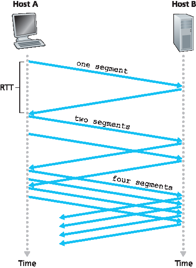
图 3.50 TCP 慢启动
但何时结束指数增长?慢启动提供几种结束条件。首先,若发生丢包事件(即拥塞)并由超时指示,发送方将 cwnd 设为 1,重新开始慢启动。同时将第二状态变量 ssthresh (慢启动阈值)设为丢包时 cwnd 的一半。第二种结束方式与 ssthresh 值相关。当 cwnd 达到或超过 ssthresh 时,停止慢启动,进入拥塞避免模式。正如后续将见,拥塞避免阶段 cwnd 增长更为谨慎。第三种结束方式是检测到三个重复 ACK,TCP 执行快速重传(参见 第3.5.4节),并进入快速恢复状态。TCP 慢启动行为在 图3.51 的状态机中有总结。慢启动算法最初见于 [Jacobson 1988];类似方法也独立由 [Jain 1986] 提出。
When a TCP connection begins, the value of cwnd is typically initialized to a small value of 1 MSS [RFC 3390], resulting in an initial sending rate of roughly MSS/RTT. For example, if MSS = 500 bytes and RTT = 200 msec, the resulting initial sending rate is only about 20 kbps. Since the available bandwidth to the TCP sender may be much larger than MSS/RTT, the TCP sender would like to find the amount of available bandwidth quickly. Thus, in the slow-start state, the value of cwnd begins at 1 MSS and increases by 1 MSS every time a transmitted segment is first acknowledged. In the example of Figure 3.50, TCP sends the first segment into the network and waits for an acknowledgment. When this acknowledgment arrives, the TCP sender increases the congestion window by one MSS and sends out two maximum-sized segments. These segments are then acknowledged, with the sender increasing the congestion window by 1 MSS for each of the acknowledged segments, giving a congestion window of 4 MSS, and so on. This process results in a doubling of the sending rate every RTT. Thus, the TCP send rate starts slow but grows exponentially during the slow start phase.
Figure 3.50 TCP slow start
But when should this exponential growth end? Slow start provides several answers to this question. First, if there is a loss event (i.e., congestion) indicated by a timeout, the TCP sender sets the value of cwnd to 1 and begins the slow start process anew. It also sets the value of a second state variable, ssthresh (shorthand for “slow start threshold”) to cwnd/2—half of the value of the congestion window value when congestion was detected. The second way in which slow start may end is directly tied to the value of ssthresh. Since ssthresh is half the value of cwnd when congestion was last detected, it might be a bit reckless to keep doubling cwnd when it reaches or surpasses the value of ssthresh. Thus, when the value of cwnd equals ssthresh, slow start ends and TCP transitions into congestion avoidance mode. As we’ll see, TCP increases cwnd more cautiously when in congestion-avoidance mode. The final way in which slow start can end is if three duplicate ACKs are detected, in which case TCP performs a fast retransmit (see Section 3.5.4) and enters the fast recovery state, as discussed below. TCP’s behavior in slow start is summarized in the FSM description of TCP congestion control in Figure 3.51. The slow-start algorithm traces it roots to [Jacobson 1988]; an approach similar to slow start was also proposed independently in [Jain 1986].
拥塞避免#
Congestion Avoidance
进入拥塞避免状态时, cwnd 约为上次拥塞时的 cwnd 一半——拥塞可能随时发生!因此 TCP 不再每 RTT 翻倍 cwnd,而是更保守地每 RTT 只增加 1 MSS [RFC 5681]。这可通过多种方式实现。常见方法是每收到一个新确认, cwnd 增加 MSS/cwnd 字节。例如,若 MSS 为 1460 字节, cwnd 为 14600 字节,则每 RTT 发送 10 个分段。每个 ACK(假设每个分段对应一个 ACK)使 cwnd 增加 1/10 MSS,因此收到全部 10 个 ACK 后 cwnd 增加 1 MSS。
那么何时结束拥塞避免的线性增长(每 RTT 增加 1 MSS)?拥塞避免算法在发生超时时表现与慢启动相同:将 cwnd 设为 1 MSS,更新 ssthresh 为丢包事件时 cwnd 的一半。需要注意的是,丢包事件也可由三次重复 ACK 触发。
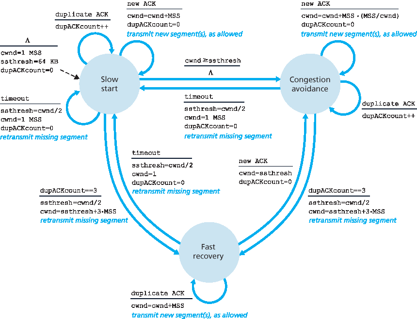
图 3.51 TCP 拥塞控制的状态机描述
在这种情况下,网络继续将分段从发送方传递到接收方(由重复 ACK 显示)。因此 TCP 对此类丢包事件的响应应比超时指示的丢包更温和:TCP 将 cwnd 减半(并为三个重复 ACK 适当增加 3 MSS),并将 ssthresh 记录为收到三次重复 ACK 时 cwnd 的一半。随后进入快速恢复状态。
On entry to the congestion-avoidance state, the value of cwnd is approximately half its value when congestion was last encountered—congestion could be just around the corner! Thus, rather than
doubling the value of cwnd every RTT, TCP adopts a more conservative approach and increases the value of cwnd by just a single MSS every RTT [RFC 5681]. This can be accomplished in several ways. A common approach is for the TCP sender to increase cwnd by MSS bytes (MSS/cwnd) whenever a
new acknowledgment arrives. For example, if MSS is 1,460 bytes and cwnd is 14,600 bytes, then 10 segments are being sent within an RTT. Each arriving ACK (assuming one ACK per segment) increases the congestion window size by 1/10 MSS, and thus, the value of the congestion window will have increased by one MSS after ACKs when all 10 segments have been received.
But when should congestion avoidance’s linear increase (of 1 MSS per RTT) end? TCP’s congestion- avoidance algorithm behaves the same when a timeout occurs. As in the case of slow start: The value of cwnd is set to 1 MSS, and the value of ssthresh is updated to half the value of cwnd when the loss event occurred. Recall, however, that a loss event also can be triggered by a triple duplicate ACK event.
Figure 3.51 FSM description of TCP congestion control
In this case, the network is continuing to deliver segments from sender to receiver (as indicated by the receipt of duplicate ACKs). So TCP’s behavior to this type of loss event should be less drastic than with a timeout-indicated loss: TCP halves the value of cwnd (adding in 3 MSS for good measure to account for the triple duplicate ACKs received) and records the value of ssthresh to be half the value of cwnd when the triple duplicate ACKs were received. The fast-recovery state is then entered.
快速恢复#
Fast Recovery
在快速恢复阶段,对于导致 TCP 进入快速恢复状态的丢失分段,发送方每收到一个该分段的重复确认 ACK, cwnd 就增加 1 MSS。当最终收到该丢失分段的确认 ACK 后,TCP 对 cwnd 进行缩减并进入拥塞避免状态。如果发生超时事件,快速恢复将在执行与慢启动和拥塞避免相同的操作后,转入慢启动状态:将 cwnd 设为 1 MSS, ssthresh 设为丢包事件发生时 cwnd 的一半。

TCP 行为考察
实践中的原则
TCP 拆分:优化云服务性能
对于搜索、电子邮件和社交网络等云服务,期望提供高响应性,理想情况下让用户感觉服务就在其终端设备(包括智能手机)上运行。这是一个重大挑战,因为用户往往距离负责提供云服务动态内容的数据中心较远。若终端系统远离数据中心,RTT 较大,TCP 慢启动可能导致响应时间较差。
以搜索查询响应延迟为例。服务器通常需要三个 TCP 窗口的时间来完成慢启动并交付响应 [Pathak 2010]。因此,从终端系统发起 TCP 连接到收到最后一个响应数据包,时间大约是 4×RTT(一个 RTT 建立连接,三个 RTT 传输数据)加上数据中心处理时间。此 RTT 延迟会导致部分查询的搜索结果返回明显延迟。此外,接入网络中可能存在大量丢包,导致 TCP 重传和更大延迟。
缓解此问题、提升用户感知性能的一种方法是:(1) 在用户附近部署前端服务器,(2) 利用 TCP 拆分,即在前端服务器处拆分 TCP 连接。通过 TCP 拆分,客户端与邻近前端建立 TCP 连接,前端与数据中心维持一个具有非常大拥塞窗口的持久 TCP 连接 [Tariq 2008,Pathak 2010,Chen 2011]。这样响应时间约为 4×RTT_FE + RTT_BE + 处理时间,其中 RTT_FE 是客户端与前端服务器之间往返时延,RTT_BE 是前端服务器与数据中心之间往返时延。如果前端服务器靠近客户端,RTT_FE 可忽略不计,RTT_BE 近似 RTT,总响应时间约为 RTT 加处理时间。总结来说,TCP 拆分将网络延迟从约 4xRTT 降至约 RTT,大幅提升用户感知性能,尤其对距离最近数据中心较远的用户效果明显。TCP 拆分还能减少因接入网络丢包导致的 TCP 重传延迟。谷歌和 Akamai 广泛利用其接入网络的 CDN 服务器(参考 第2.6节)对所支持的云服务进行 TCP 拆分 [Chen 2011]。
快速恢复是 TCP RFC 5681 推荐但非强制的组成部分。有趣的是,TCP 早期版本 TCP Tahoe 在超时或三次重复 ACK 指示丢包事件后,无条件将拥塞窗口缩减至 1 MSS 并进入慢启动阶段。较新版本 TCP Reno 则引入了快速恢复机制。
图3.52 展示了 TCP Reno 和 Tahoe 的拥塞窗口演变过程。图中阈值初始为 8 MSS。前八个传输轮次中,Tahoe 和 Reno 动作相同。慢启动阶段拥塞窗口指数增长,并在第 4 轮达到阈值。此后拥塞窗口线性增长,直到第 8 轮传输后出现三次重复 ACK 事件。丢包事件发生时拥塞窗口为 12xMSS。ssthresh 被设为 0.5×cwnd = 6 MSS。在 TCP Reno 中,拥塞窗口被设为 cwnd =9 MSS,随后线性增长。TCP Tahoe 中,拥塞窗口被设为 1 MSS,指数增长直至达到 ssthresh,此后线性增长。
图3.51 展示了 TCP 拥塞控制算法(慢启动、拥塞避免和快速恢复)的完整状态机描述。图中还指示了新分段或重传分段的发送时机。尽管区分 TCP 错误控制/重传和拥塞控制很重要,但也应理解这两者如何紧密关联。
In fast recovery, the value of cwnd is increased by 1 MSS for every duplicate ACK received for the missing segment that caused TCP to enter the fast-recovery state. Eventually, when an ACK arrives for the missing segment, TCP enters the congestion-avoidance state after deflating cwnd. If a timeout event occurs, fast recovery transitions to the slow-start state after performing the same actions as in slow start and congestion avoidance: The value of cwnd is set to 1 MSS, and the value of ssthresh is set to half the value of cwnd when the loss event occurred.
Examining the behavior of TCP
PRINCIPLES IN PRACTICE
TCP SPLITTING: OPTIMIZING THE PERFORMANCE OF CLOUD SERVICES
For cloud services such as search, e-mail, and social networks, it is desirable to provide a high- level of responsiveness, ideally giving users the illusion that the services are running within their own end systems (including their smartphones). This can be a major challenge, as users are often located far away from the data centers responsible for serving the dynamic content associated with the cloud services. Indeed, if the end system is far from a data center, then the RTT will be large, potentially leading to poor response time performance due to TCP slow start.
As a case study, consider the delay in receiving a response for a search query. Typically, the server requires three TCP windows during slow start to deliver the response [Pathak 2010]. Thus the time from when an end system initiates a TCP connection until the time when it receives the last packet of the response is roughly 4⋅RTT (one RTT to set up the TCP connection plus three RTTs for the three windows of data) plus the processing time in the data center. These RTT delays can lead to a noticeable delay in returning search results for a significant fraction of queries. Moreover, there can be significant packet loss in access networks, leading to TCP retransmissions and even larger delays.
One way to mitigate this problem and improve user-perceived performance is to (1) deploy front- end servers closer to the users, and (2) utilize TCP splitting by breaking the TCP connection at the front-end server. With TCP splitting, the client establishes a TCP connection to the nearby front-end, and the front-end maintains a persistent TCP connection to the data center with a very large TCP congestion window [Tariq 2008, Pathak 2010, Chen 2011]. With this approach, the response time roughly becomes 4⋅RTTFE+RTTBE+ processing time, where RTTFE is the round- trip time between client and front-end server, and RTTBE is the round-trip time between the front- end server and the data center (back-end server). If the front-end server is close to client, then this response time approximately becomes RTT plus processing time, since RTTFE is negligibly small and RTTBE is approximately RTT. In summary, TCP splitting can reduce the networking delay roughly from 4⋅RTT to RTT, significantly improving user-perceived performance, particularly for users who are far from the nearest data center. TCP splitting also helps reduce TCP retransmission delays caused by losses in access networks. Google and Akamai have made extensive use of their CDN servers in access networks (recall our discussion in Section 2.6) to perform TCP splitting for the cloud services they support [Chen 2011].
Fast recovery is a recommended, but not required, component of TCP RFC 5681. It is interesting that an early version of TCP, known as TCP Tahoe, unconditionally cut its congestion window to 1 MSS and entered the slow-start phase after either a timeout-indicated or triple-duplicate-ACK-indicated loss event. The newer version of TCP, TCP Reno, incorporated fast recovery.
Figure 3.52 illustrates the evolution of TCP’s congestion window for both Reno and Tahoe. In this figure, the threshold is initially equal to 8 MSS. For the first eight transmission rounds, Tahoe and Reno take identical actions. The congestion window climbs exponentially fast during slow start and hits the threshold at the fourth round of transmission. The congestion window then climbs linearly until a triple duplicate- ACK event occurs, just after transmission round 8. Note that the congestion window is 12⋅MSS when this loss event occurs. The value of ssthresh is then set to 0.5⋅ cwnd =6⋅MSS. Under TCP Reno, the congestion window is set to cwnd = 9⋅MSS and then grows linearly. Under TCP Tahoe, the congestion window is set to 1 MSS and grows exponentially until it reaches the value of ssthresh, at which point it grows linearly.
Figure 3.51 presents the complete FSM description of TCP’s congestion-control algorithms—slow start, congestion avoidance, and fast recovery. The figure also indicates where transmission of new segments or retransmitted segments can occur. Although it is important to distinguish between TCP error control/retransmission and TCP congestion control, it’s also important to appreciate how these two aspects of TCP are inextricably linked.
TCP 拥塞控制回顾#
TCP Congestion Control: Retrospective
深入了解慢启动、拥塞避免和快速恢复后,值得退一步,全面审视全貌。忽略连接开始时的慢启动阶段,假设丢包由三次重复 ACK 指示而非超时,TCP 拥塞控制表现为每 RTT 线性(加法)增加 cwnd 1 MSS,在三次重复 ACK 事件时将 cwnd 减半(乘法减小)。因此,TCP 拥塞控制常被称为 加法增大,乘法减小(AIMD)。AIMD 拥塞控制导致 图3.53 所示的“锯齿”行为,也很好地体现了我们先前对 TCP 进行带宽“探测”的直觉——TCP 线性增加拥塞窗口(及发送速率),直至发生三次重复 ACK,随后将拥塞窗口缩减一半,再次线性增加,继续探测可用带宽。
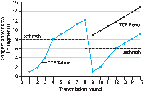
图 3.52 TCP 拥塞窗口演变(Tahoe 和 Reno)
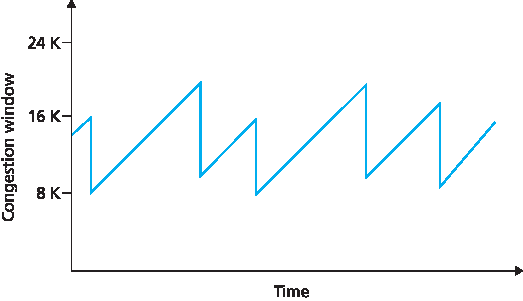
图 3.53 加法增大,乘法减小拥塞控制
如前所述,许多 TCP 实现采用 Reno 算法 [Padhye 2001]。Reno 算法有多种变体 [RFC 3782;RFC 2018]。TCP Vegas 算法 [Brakmo 1995;Ahn 1995] 试图避免拥塞同时保持良好吞吐量。Vegas 的基本思路是:(1) 在源到目的地的路由器中,在丢包发生前检测拥塞;(2) 预测即将发生丢包时线性降低发送速率。通过观察 RTT 预测即将发生的丢包,RTT 越长,路由器拥塞越严重。截至 2015 年末,Ubuntu Linux TCP 实现默认支持慢启动、拥塞避免、快速恢复、快速重传和选择确认(SACK);同时也提供如 TCP Vegas 和 BIC [Xu 2004] 等替代拥塞控制算法。有关 TCP 多种变体的综述,参见 [Afanasyev 2010]。
TCP 的 AIMD 算法基于大量工程洞察和在实际网络中的拥塞控制实验开发。TCP 开发十年后,理论分析表明 TCP 拥塞控制算法作为分布式异步优化算法,能同时优化用户和网络性能的多个重要方面 [Kelly 1998]。此后,拥塞控制理论得到了丰富发展 [Srikant 2004]。
Having delved into the details of slow start, congestion avoidance, and fast recovery, it’s worthwhile to now step back and view the forest from the trees. Ignoring the initial slow-start period when a connection begins and assuming that losses are indicated by triple duplicate ACKs rather than timeouts, TCP’s congestion control consists of linear (additive) increase in cwnd of 1 MSS per RTT and then a halving (multiplicative decrease) of cwnd on a triple duplicate-ACK event. For this reason, TCP congestion control is often referred to as an additive-increase, multiplicative-decrease (AIMD) form of congestion control. AIMD congestion control gives rise to the “saw tooth” behavior shown in Figure 3.53, which also nicely illustrates our earlier intuition of TCP “probing” for bandwidth—TCP linearly increases its congestion window size (and hence its transmission rate) until a triple duplicate-ACK event occurs. It then decreases its congestion window size by a factor of two but then again begins increasing it linearly, probing to see if there is additional available bandwidth.
Figure 3.52 Evolution of TCP’s congestion window (Tahoe and Reno)
Figure 3.53 Additive-increase, multiplicative-decrease congestion control
As noted previously, many TCP implementations use the Reno algorithm [Padhye 2001]. Many variations of the Reno algorithm have been proposed [RFC 3782; RFC 2018]. The TCP Vegas algorithm [Brakmo 1995; Ahn 1995] attempts to avoid congestion while maintaining good throughput. The basic idea of Vegas is to (1) detect congestion in the routers between source and destination before packet loss occurs, and (2) lower the rate linearly when this imminent packet loss is detected. Imminent packet loss is predicted by observing the RTT. The longer the RTT of the packets, the greater the congestion in the routers. As of late 2015, the Ubuntu Linux implementation of TCP provided slowstart, congestion avoidance, fast recovery, fast retransmit, and SACK, by default; alternative congestion control algorithms, such as TCP Vegas and BIC [Xu 2004], are also provided. For a survey of the many flavors of TCP, see [Afanasyev 2010].
TCP’s AIMD algorithm was developed based on a tremendous amount of engineering insight and experimentation with congestion control in operational networks. Ten years after TCP’s development, theoretical analyses showed that TCP’s congestion-control algorithm serves as a distributed asynchronous-optimization algorithm that results in several important aspects of user and network performance being simultaneously optimized [Kelly 1998]. A rich theory of congestion control has since been developed [Srikant 2004].
TCP 吞吐量的宏观描述#
Macroscopic Description of TCP Throughput
鉴于 TCP 的锯齿行为,自然想要分析长连接的平均吞吐量(即平均速率)。本分析忽略超时事件后的慢启动阶段(该阶段通常很短,因为发送方指数增长快速跳出该阶段)。在特定往返时延区间内,TCP 发送数据速率由拥塞窗口大小和当前 RTT 决定。当窗口大小为 w 字节,RTT 为 RTT 秒时,TCP 发送速率约为 w/RTT。TCP 通过每 RTT 增加 1 MSS 来探测额外带宽,直到发生丢包事件。设丢包时窗口大小为 W。假设 RTT 和 W 在连接期间大致保持不变,则 TCP 发送速率在 W/(2·RTT) 到 W/RTT 之间波动。该假设导出 TCP 稳态行为的极简宏观模型。当发送速率达到 W/RTT 时网络丢包,速率减半,然后每 RTT 增加 MSS/RTT,直至再次达到 W/RTT。该过程不断重复。因 TCP 发送速率在线性变化区间内均匀增加,故有:
连接平均吞吐量 = 0.75 x W / RTT
基于此高度理想化的 TCP 稳态模型,我们还能推导出连接丢包率与可用带宽的关系式 [Mahdavi 1997]。推导见作业题目。一个经验上与测量数据吻合更好的复杂模型见 [Padhye 2000]。
Given the saw-toothed behavior of TCP, it’s natural to consider what the average throughput (that is, the average rate) of a long-lived TCP connection might be. In this analysis we’ll ignore the slow-start phases that occur after timeout events. (These phases are typically very short, since the sender grows out of the phase exponentially fast.) During a particular round-trip interval, the rate at which TCP sends data is a function of the congestion window and the current RTT. When the window size is w bytes and the current round-trip time is RTT seconds, then TCP’s transmission rate is roughly w/RTT. TCP then probes for additional bandwidth by increasing w by 1 MSS each RTT until a loss event occurs. Denote by W the value of w when a loss event occurs. Assuming that RTT and W are approximately constant over the duration of the connection, the TCP transmission rate ranges from W/(2 · RTT) to W/RTT. These assumptions lead to a highly simplified macroscopic model for the steady-state behavior of TCP. The network drops a packet from the connection when the rate increases to W/RTT; the rate is then cut in half and then increases by MSS/RTT every RTT until it again reaches W/RTT. This process repeats itself over and over again. Because TCP’s throughput (that is, rate) increases linearly between the two extreme values, we have
average throughput of a connection=0.75⋅WRTT
Using this highly idealized model for the steady-state dynamics of TCP, we can also derive an interesting expression that relates a connection’s loss rate to its available bandwidth [Mahdavi 1997]. This derivation is outlined in the homework problems. A more sophisticated model that has been found empirically to agree with measured data is [Padhye 2000].
TCP 在高带宽路径上的表现#
TCP Over High-Bandwidth Paths
需要认识到的是,TCP 拥塞控制多年来不断发展,并且仍在持续演进。关于当前 TCP 变体的总结以及 TCP 演进的讨论,请参见 [ Floyd 2001,RFC 5681,Afanasyev 2010]。在以 SMTP、FTP 和 Telnet 流量为主的时代,适合互联网的 TCP 方式,并不一定适合今日以 HTTP 为主导的互联网,或者未来那些尚未预见到的服务。
TCP 需要持续演进的需求,可以通过考虑网格计算和云计算应用所需的高速 TCP 连接来说明。例如,考虑一个 MSS 为 1500 字节,RTT 为 100 毫秒的 TCP 连接,假设我们希望通过该连接发送 10 Gbps 的数据。根据 [RFC 3649],利用前文的 TCP 吞吐量公式,为达到 10 Gbps 的吞吐量,平均拥塞窗口大小需要为 83,333 个分段。这个数量极大,使得我们非常担心这 83,333 个在途分段中某个分段可能丢失。若发生丢包,会有什么影响?换句话说,允许 TCP 拥塞控制算法(如 图3.51 所示)仍能实现 10 Gbps 速率的最大丢包率是多少?本章作业题将引导你推导一个公式,将 TCP 连接的吞吐量与丢包率 (L)、往返时延 (RTT) 和最大分段大小 (MSS) 关联起来:
连接平均吞吐量 = 1.22 x MSS / (RTT x √L)
利用该公式,我们看到要实现 10 Gbps 的吞吐量,现有 TCP 拥塞控制算法只能容忍约 \(2 · 10^{–10}\) 的分段丢包概率(即每 50 亿个分段发生一次丢包事件)——这是极低的丢包率。该观察促使众多研究者探索专门针对高速环境设计的新 TCP 版本;相关讨论见 [ Jin 2004;Kelly 2003;Ha 2008;RFC 7323]。
It is important to realize that TCP congestion control has evolved over the years and indeed continues to evolve. For a summary of current TCP variants and discussion of TCP evolution, see [ Floyd 2001, RFC 5681, Afanasyev 2010]. What was good for the Internet when the bulk of the TCP connections carried SMTP, FTP, and Telnet traffic is not necessarily good for today’s HTTP-dominated Internet or for a future Internet with services that are still undreamed of.
The need for continued evolution of TCP can be illustrated by considering the high-speed TCP connections that are needed for grid- and cloud-computing applications. For example, consider a TCP connection with 1,500-byte segments and a 100 ms RTT, and suppose we want to send data through this connection at 10 Gbps. Following [RFC 3649], we note that using the TCP throughput formula above, in order to achieve a 10 Gbps throughput, the average congestion window size would need to be 83,333 segments. That’s a lot of segments, leading us to be rather concerned that one of these 83,333 in-flight segments might be lost. What would happen in the case of a loss? Or, put another way, what fraction of the transmitted segments could be lost that would allow the TCP congestion-control algorithm specified in Figure 3.51 still to achieve the desired 10 Gbps rate? In the homework questions for this chapter, you are led through the derivation of a formula relating the throughput of a TCP connection as a function of the loss rate (L), the round-trip time (RTT), and the maximum segment size (MSS):
average throughput of a connection=1.22⋅MSSRTTL
Using this formula, we can see that in order to achieve a throughput of 10 Gbps, today’s TCP congestion-control algorithm can only tolerate a segment loss probability of \(2 · 10^{–10}\) (or equivalently, one loss event for every 5,000,000,000 segments)—a very low rate. This observation has led a number of researchers to investigate new versions of TCP that are specifically designed for such high-speed environments; see [ Jin 2004; Kelly 2003; Ha 2008; RFC 7323] for discussions of these efforts.
3.7.2 公平性#
3.7.2 Fairness
考虑 K 个 TCP 连接,每个连接经过不同的端到端路径,但都通过一个传输速率为 R bps 的瓶颈链路。(所谓 瓶颈链路 ,是指对于每个连接,其路径上除该链路外的其他链路均未拥塞,且传输能力远大于该瓶颈链路。)假设每个连接都在传输大型文件,且瓶颈链路上没有 UDP 流量。若拥塞控制机制能使每个连接的平均传输速率约为 R/K,则称该机制是公平的;即每个连接平等分享链路带宽。
TCP 的 AIMD 算法是否公平?尤其是考虑不同 TCP 连接可能在不同时间启动,因而在某一时刻拥有不同的窗口大小?[Chiu 1989] 提供了对 TCP 拥塞控制为何最终收敛至竞争 TCP 连接间平等分享瓶颈链路带宽的优雅且直观的解释。
让我们考虑两个 TCP 连接共享一条传输速率为 R 的链路的简单情况,如 图3.54 所示。假设两个连接具有相同的 MSS 和 RTT(因此拥塞窗口相同时吞吐量相同),且有大量数据待发送,没有其他 TCP 连接或 UDP 数据报经过该共享链路。忽略 TCP 的慢启动阶段,假设 TCP 连接始终处于拥塞避免(CA)模式(AIMD)。
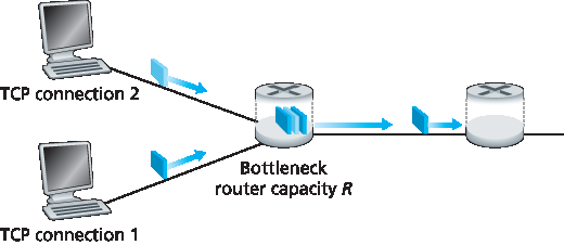
图 3.54 两个 TCP 连接共享单一瓶颈链路
图3.55 绘出了两个 TCP 连接实现的吞吐量。如果 TCP 要在两个连接间公平分享链路带宽,则实现的吞吐量应落在从原点发出的 45 度箭头线上(表示带宽均分)。理想情况下,两者吞吐量之和应为 R。(当然,每个连接都获得等量但为零的带宽份额显然不可取!)因此目标是使实现的吞吐量落在 图3.55 中的均分线与满载线交点附近。
假设 TCP 窗口大小使得某时刻连接 1 和 2 的吞吐量对应 图3.55 中的点 A。由于两连接联合消耗的链路带宽小于 R,不会发生丢包,两个连接会根据 TCP 拥塞避免算法每 RTT 各增加 1 MSS 窗口大小。于是两连接的总吞吐量沿着从点 A 出发的 45 度线(两连接均等增长)前进。最终两连接联合消耗的带宽将超过 R,导致丢包发生。假设丢包发生时吞吐量对应点 B,连接 1 和 2 随后窗口减半,吞吐量变为点 C(在点 B 和原点的连线中点)。由于点 C 联合带宽小于 R,两连接再次沿从 C 出发的 45 度线增加吞吐量。丢包随后再次发生,如点 D,窗口再次减半,循环往复。你应确信,两连接实现的带宽最终围绕均分线波动;无论初始点位于二维空间何处,两连接最终都会趋于这种行为。尽管该场景基于许多理想假设,但直观体现了为何 TCP 连接间能实现带宽平分。
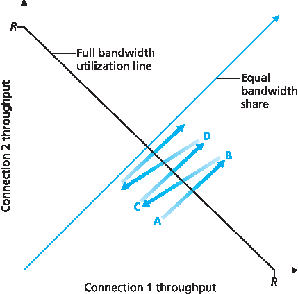
图 3.55 TCP 连接 1 和 2 的实现吞吐量
在我们的理想化场景中,假设只有 TCP 连接经过瓶颈链路,且连接 RTT 相同,并且每对主机-目的地仅对应一个 TCP 连接。实际情况通常不满足这些条件,因此客户端-服务器应用获得的链路带宽份额差异较大。尤其已知当多个连接共享瓶颈时,RTT 较小的会更快抢占链路带宽(即更快打开拥塞窗口),因此吞吐量高于 RTT 较大的连接 [Lakshman 1997]。
Consider K TCP connections, each with a different end-to-end path, but all passing through a bottleneck link with transmission rate R bps. (By bottleneck link, we mean that for each connection, all the other links along the connection’s path are not congested and have abundant transmission capacity as compared with the transmission capacity of the bottleneck link.) Suppose each connection is transferring a large file and there is no UDP traffic passing through the bottleneck link. A congestion-control mechanism is said to be fair if the average transmission rate of each connection is approximately R/K; that is, each connection gets an equal share of the link bandwidth.
Is TCP’s AIMD algorithm fair, particularly given that different TCP connections may start at different times and thus may have different window sizes at a given point in time? [Chiu 1989] provides an elegant and intuitive explanation of why TCP congestion control converges to provide an equal share of a bottleneck link’s bandwidth among competing TCP connections.
Let’s consider the simple case of two TCP connections sharing a single link with transmission rate R, as shown in Figure 3.54. Assume that the two connections have the same MSS and RTT (so that if they have the same congestion window size, then they have the same throughput), that they have a large amount of data to send, and that no other TCP connections or UDP datagrams traverse this shared link. Also, ignore the slow-start phase of TCP and assume the TCP connections are operating in CA mode (AIMD) at all times.
Figure 3.54 Two TCP connections sharing a single bottleneck link
Figure 3.55 plots the throughput realized by the two TCP connections. If TCP is to share the link bandwidth equally between the two connections, then the realized throughput should fall along the 45-degree arrow (equal bandwidth share) emanating from the origin. Ideally, the sum of the two throughputs should equal R. (Certainly, each connection receiving an equal, but zero, share of the link capacity is not a desirable situation!) So the goal should be to have the achieved throughputs fall somewhere near the intersection of the equal bandwidth share line and the full bandwidth utilization line in Figure 3.55.
Suppose that the TCP window sizes are such that at a given point in time, connections 1 and 2 realize throughputs indicated by point A in Figure 3.55. Because the amount of link bandwidth jointly consumed by the two connections is less than R, no loss will occur, and both connections will increase their window by 1 MSS per RTT as a result of TCP’s congestion-avoidance algorithm. Thus, the joint throughput of the two connections proceeds along a 45-degree line (equal increase for both connections) starting from point A. Eventually, the link bandwidth jointly consumed by the two connections will be greater than R, and eventually packet loss will occur. Suppose that connections 1 and 2 experience packet loss when they realize throughputs indicated by point B. Connections 1 and 2 then decrease their windows by a factor of two. The resulting throughputs realized are thus at point C, halfway along a vector starting at B and ending at the origin. Because the joint bandwidth use is less than R at point C, the two connections again increase their throughputs along a 45-degree line starting from C. Eventually, loss will again occur, for example, at point D, and the two connections again decrease their window sizes by a factor of two, and so on. You should convince yourself that the bandwidth realized by the two connections eventually fluctuates along the equal bandwidth share line. You should also convince yourself that the two connections will converge to this behavior regardless of where they are in the two- dimensional space! Although a number of idealized assumptions lie behind this scenario, it still provides an intuitive feel for why TCP results in an equal sharing of bandwidth among connections.
Figure 3.55 Throughput realized by TCP connections 1 and 2
In our idealized scenario, we assumed that only TCP connections traverse the bottleneck link, that the connections have the same RTT value, and that only a single TCP connection is associated with a host- destination pair. In practice, these conditions are typically not met, and client-server applications can thus obtain very unequal portions of link bandwidth. In particular, it has been shown that when multiple connections share a common bottleneck, those sessions with a smaller RTT are able to grab the available bandwidth at that link more quickly as it becomes free (that is, open their congestion windows faster) and thus will enjoy higher throughput than those connections with larger RTTs [Lakshman 1997].
公平性与 UDP#
Fairness and UDP
我们刚才看到 TCP 拥塞控制如何通过拥塞窗口机制调节应用传输速率。许多多媒体应用,如互联网电话和视频会议,常不使用 TCP,原因正是它们不希望被限制传输速率,即使网络严重拥塞。相反,这些应用倾向使用无拥塞控制的 UDP。运行于 UDP 上时,应用以恒定速率发送音视频流,偶尔丢包,而不是在拥塞时降低速率至“公平”水平以避免丢包。对 TCP 来说,运行于 UDP 上的多媒体应用不公平——它们不与其他连接协作,也不适当调整传输速率。由于 TCP 拥塞控制会在拥塞(丢包)时降低速率,而 UDP 流量不受此限制,UDP 流可能挤占 TCP 流量。当前研究领域之一是开发能防止 UDP 流量令互联网吞吐骤降的拥塞控制机制 [Floyd 1999;Floyd 2000;Kohler 2006;RFC 4340]。
We have just seen how TCP congestion control regulates an application’s transmission rate via the congestion window mechanism. Many multimedia applications, such as Internet phone and video conferencing, often do not run over TCP for this very reason—they do not want their transmission rate throttled, even if the network is very congested. Instead, these applications prefer to run over UDP, which does not have built-in congestion control. When running over UDP, applications can pump their audio and video into the network at a constant rate and occasionally lose packets, rather than reduce their rates to “fair” levels at times of congestion and not lose any packets. From the perspective of TCP, the multimedia applications running over UDP are not being fair—they do not cooperate with the other connections nor adjust their transmission rates appropriately. Because TCP congestion control will decrease its transmission rate in the face of increasing congestion (loss), while UDP sources need not, it is possible for UDP sources to crowd out TCP traffic. An area of research today is thus the development of congestion-control mechanisms for the Internet that prevent UDP traffic from bringing the Internet’s throughput to a grinding halt [Floyd 1999; Floyd 2000; Kohler 2006; RFC 4340].
公平性与并行 TCP 连接#
Fairness and Parallel TCP Connections
即使我们能强制 UDP 流量公平行为,公平性问题仍未完全解决。原因是无法阻止基于 TCP 的应用使用多条并行连接。例如,网页浏览器常用多条并行 TCP 连接传输网页中的多个对象。(多数浏览器允许配置并行连接数量。)当应用使用多条并行连接时,会在拥塞链路中获得更大带宽份额。举例来说,考虑传输速率为 R 的链路,有九个客户端-服务器应用各用一条 TCP 连接。如果新应用也使用一条 TCP 连接,每个应用获得大约 R/10 的传输速率。但若新应用改用 11 条并行 TCP 连接,则新应用获得超过 R/2 的不公平带宽份额。鉴于网页流量在互联网中的普遍性,多条并行连接并不罕见。
But even if we could force UDP traffic to behave fairly, the fairness problem would still not be completely solved. This is because there is nothing to stop a TCP-based application from using multiple parallel connections. For example, Web browsers often use multiple parallel TCP connections to transfer the multiple objects within a Web page. (The exact number of multiple connections is configurable in most browsers.) When an application uses multiple parallel connections, it gets a larger fraction of the bandwidth in a congested link. As an example, consider a link of rate R supporting nine ongoing client- server applications, with each of the applications using one TCP connection. If a new application comes along and also uses one TCP connection, then each application gets approximately the same transmission rate of R/10. But if this new application instead uses 11 parallel TCP connections, then the new application gets an unfair allocation of more than R/2. Because Web traffic is so pervasive in the Internet, multiple parallel connections are not uncommon.
3.7.3 显式拥塞通知(ECN):网络辅助拥塞控制#
3.7.3 Explicit Congestion Notification (ECN): Network-assisted Congestion Control
自 1980 年代末慢启动和拥塞避免首次标准化以来 RFC 1122,TCP 实现了我们在 第3.7.1节 研究的端到端拥塞控制形式:TCP 发送方不从网络层获得显式拥塞指示,而是通过观察丢包间接推断拥塞。近期,IP 和 TCP 的扩展 [RFC 3168] 被提议、实现并部署,使网络能显式向 TCP 发送和接收端信号拥塞状态。这种网络辅助拥塞控制称为 显式拥塞通知(ECN) 。如 图3.56 所示,TCP 和 IP 协议共同参与。
在网络层,IP 数据报头的服务类型字段(将在 第4.3节 讨论)中使用了两位(二进制四种取值)作为 ECN 标志。路由器用 ECN 位的某种设置表示自己正经历拥塞。该拥塞指示随被标记的数据报送达目的主机,目的主机随后通知发送主机,如 图3.56 所示。RFC 3168 未定义何时视路由器为拥塞状态;该决策由路由器厂商配置,网络运营商决定。然而,RFC 3168 建议仅在持续拥塞时设置 ECN 拥塞标志。ECN 位的另一种设置由发送主机用来告知路由器发送和接收端均支持 ECN,并能响应 ECN 网络拥塞指示。
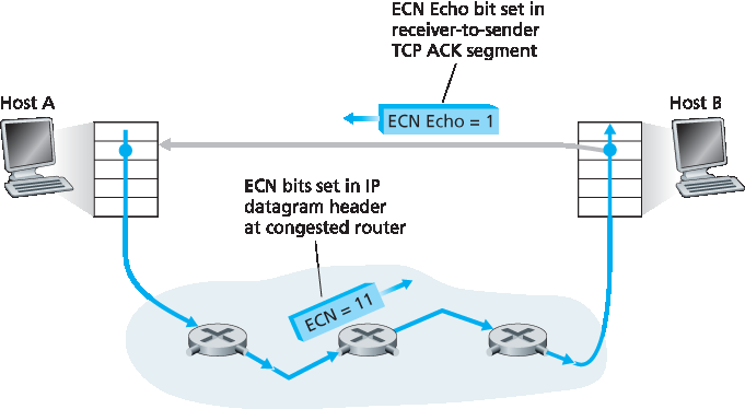
图 3.56 显式拥塞通知:网络辅助拥塞控制
如 图3.56 所示,接收端 TCP 通过收到带有 ECN 拥塞标记的数据报获知拥塞后,接收端 TCP 通过在发往发送端的 TCP ACK 段中设置 ECE(显式拥塞通知回显)位(参见 图3.29)告知发送端。发送端 TCP 收到带有 ECE 标志的 ACK 后,响应方式与快速重传时遇丢包相同,将拥塞窗口减半,并在下一次发送的 TCP 段头中设置 CWR(拥塞窗口减小)位。
除 TCP 外,其他传输层协议也可利用网络层的 ECN 信号。数据报拥塞控制协议(DCCP) [RFC 4340] 提供低开销、拥塞控制的类似 UDP 的不可靠服务,利用 ECN。专为数据中心网络设计的 DCTCP(数据中心 TCP) [Alizadeh 2010] 也使用 ECN。
Since the initial standardization of slow start and congestion avoidance in the late 1980’s RFC 1122, TCP has implemented the form of end-end congestion control that we studied in Section 3.7.1: a TCP sender receives no explicit congestion indications from the network layer, and instead infers congestion through observed packet loss. More recently, extensions to both IP and TCP [RFC 3168] have been proposed, implemented, and deployed that allow the network to explicitly signal congestion to a TCP sender and receiver. This form of network-assisted congestion control is known as Explicit Congestion Notification. As shown in Figure 3.56, the TCP and IP protocols are involved.
At the network layer, two bits (with four possible values, overall) in the Type of Service field of the IP datagram header (which we’ll discuss in Section 4.3) are used for ECN. One setting of the ECN bits is used by a router to indicate that it (the router) is experiencing congestion. This congestion indication is then carried in the marked IP datagram to the destination host, which then informs the sending host, as shown in Figure 3.56. RFC 3168 does not provide a definition of when a router is congested; that decision is a configuration choice made possible by the router vendor, and decided by the network operator. However, RFC 3168 does recommend that an ECN congestion indication be set only in the face of persistent congestion. A second setting of the ECN bits is used by the sending host to inform routers that the sender and receiver are ECN-capable, and thus capable of taking action in response to ECN-indicated network congestion.
Figure 3.56 Explicit Congestion Notification: network-assisted congestion control
As shown in Figure 3.56, when the TCP in the receiving host receives an ECN congestion indication via a received datagram, the TCP in the receiving host informs the TCP in the sending host of the congestion indication by setting the ECE (Explicit Congestion Notification Echo) bit (see Figure 3.29) in a receiver-to-sender TCP ACK segment. The TCP sender, in turn, reacts to an ACK with an ECE congestion indication by halving the congestion window, as it would react to a lost segment using fast retransmit, and sets the CWR (Congestion Window Reduced) bit in the header of the next transmitted TCP sender-to-receiver segment.
Other transport-layer protocols besides TCP may also make use of network-layer-signaled ECN. The Datagram Congestion Control Protocol (DCCP) [RFC 4340] provides a low-overhead, congestion-controlled UDP-like unreliable service that utilizes ECN. DCTCP (Data Center TCP) [Alizadeh 2010], a version of TCP designed specifically for data center networks, also makes use of ECN.