5.2 路由算法#

5.2 Routing Algorithms

在本节中，我们将学习 路由算法，其目标是在由路由器组成的网络中，为从发送端到接收端寻找良好的路径（或称“路由”）。通常意义上，“良好”的路径是代价最小的路径。然而我们也将看到，在实际应用中，还必须考虑一些现实问题，例如策略问题（例如，“属于组织 Y 的路由器 x 不应转发任何来自组织 Z 拥有的网络的数据包”）。我们注意到，无论网络控制平面采用的是每路由器控制方式还是逻辑集中控制方式，都必须有一个明确的路由器序列，数据包必须穿过该序列从发送主机到达接收主机。因此，计算这些路径的路由算法具有基础性的意义，是我们“十大基本网络概念”候选之一。

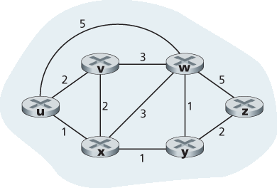
图5.3 计算机网络的抽象图模型(Abstract graph model)

图用于形式化地表示路由问题。回忆一下， 图(graph) G=(N, E) 是一个由节点集合 N 和边集合 E 组成的结构，其中每条边是 N 中两个节点的对。在网络层路由的上下文中，图中的节点代表路由器——即做出转发决策的点——而连接这些节点的边表示路由器之间的物理链路。计算机网络的这种图抽象如图 5.3 所示。要查看一些真实网络地图所对应的图，请参见 [Dodge 2016、Cheswick 2000]；要了解不同图模型对 Internet 的拟合程度，请参见 [Zegura 1997、Faloutsos 1999、Li 2004]。

如图 5.3 所示，每条边也有一个表示其代价的数值。通常，边的代价可能反映相应链路的物理长度（例如，跨洋链路的代价可能比短距离地面链路高）、链路速率，或链路的经济成本。在本节中，我们将直接采用给定的边的代价，而不考虑这些代价是如何确定的。对于 E 中的任意边 (x, y)，我们记 c(x, y) 为节点 x 和 y 之间边的代价。如果 (x, y) 不属于 E，则设 c(x, y) = ∞ 。此外，我们这里仅考虑无向图（即边没有方向），因此边 (x, y) 与 (y, x) 是相同的，并且有 c(x, y)=c(y, x)。如果 (x, y) ∈ E，则称节点 y 是节点 x 的邻居。

既然成本被分配给抽象的图中的各个边，路由算法的自然目标就是确定源和目的地之间成本最低的路径。为了更精确定义这个问题，回忆一下图 G=(N, E) 中的路径是一组节点序列 $(x_{1}, x_{2}, . . ., x_{p})$ ，使得所有相邻对 $(x_{1}, x_{2}), (x_{2}, x_{3}), . . ., (x_{p} - 1, x_{p})$ 都是 E 中的边。路径 $(x_{1}, x_{2}, . . ., x_{p})$ 的代价是该路径上所有边的代价之和，即 $c (x_{1}, x_{2}) + c (x_{2}, x_{3}) + . . . + c (x_{p} - 1, x_{p})$ 。对于任意两个节点 x 和 y，通常存在多条路径连接它们，每条路径都有其代价。其中一条或多条路径是 最小代价路径。因此，最小代价问题很明确：找出从源到目标具有最小代价的路径。例如，在图 5.3 中，从源节点 u 到目标节点 w 的最小代价路径为 (u, x, y, w)，路径代价为 3。注意，如果图中所有边的代价都相同，则最小代价路径也是 最短路径 （即源节点与目标节点之间链路数最少的路径）。

作为一个简单练习，试着在图 5.3 中找出从节点 u 到 z 的最小代价路径，并想一想你是如何计算出这条路径的。如果你像大多数人一样，你是通过观察图 5.3，尝试几条从 u 到 z 的路径，并确信自己选择的路径具有所有可能路径中最小的代价。（你检查了 u 到 z 的所有 17 条可能路径吗？可能没有！）这种计算是集中式路由算法的例子——算法在一个地方运行，你的大脑，且拥有整个网络的完整信息。从广义上讲，我们可以将路由算法根据其是集中式还是分布式进行分类。

集中式路由算法 使用对整个网络的完整全局知识计算源与目的之间的最小代价路径。即，该算法以所有节点间的连接关系和所有链路的代价为输入。这要求算法在实际计算前能够以某种方式获得这些信息。该计算可在某一个站点运行（例如图 5.2 中的逻辑集中控制器），也可以在每个路由器的路由组件中复制运行（例如图 5.1）。然而关键特征在于算法拥有完整的连接性和链路代价信息。具有全局状态信息的算法通常称为 链路状态（LS）算法，因为该算法必须知道网络中每条链路的代价。我们将在第 5.2.1 节中学习链路状态算法。
在 分布式路由算法 中，最小代价路径的计算由路由器以迭代、分布式的方式执行。没有任何一个节点拥有所有网络链路代价的完整信息。相反，每个节点起始时只知道其直连链路的代价。然后，通过与相邻节点交换信息并进行迭代计算，一个节点逐渐计算出到某个目标或目标集合的最小代价路径。我们将在第 5.2.2 节中学习的分布式路由算法被称为距离向量（DV）算法，因为每个节点维护一张估计到网络中所有其他节点代价（距离）的向量。这类分布式算法通过邻居路由器间的交互消息交换，也许更自然地适用于如图 5.1 中所示的控制平面，即路由器之间直接交互的控制方式。

我们还可以按静态与动态将路由算法划分为第二类。在 静态路由算法 中，路由路径随时间变化非常缓慢，通常是人工干预的结果（例如人工编辑链路代价）。而 动态路由算法 会随着网络流量负载或拓扑的变化而更改路由路径。动态算法可以定期运行，也可以在检测到拓扑或链路代价变化时立即运行。虽然动态算法对网络变化更具响应性，但也更容易遇到路由环、路由震荡等问题。

我们还可以按是否对负载敏感将路由算法划分为第三类。在 负载敏感算法 中，链路代价动态变化以反映底层链路的当前拥塞程度。如果某条链路当前拥塞并因此具有较高代价，路由算法将倾向于绕开该链路。尽管早期 ARPAnet 使用了负载敏感算法 [McQuillan 1980]，但也遇到了许多问题 [Huitema 1998]。当今互联网中的路由算法（如 RIP、OSPF 和 BGP）是 负载不敏感的，即链路的代价不会显式反映其当前或过去的拥塞程度。

原文

In this section we’ll study routing algorithms, whose goal is to determine good paths (equivalently, routes), from senders to receivers, through the network of routers. Typically, a “good” path is one that has the least cost. We’ll see that in practice, however, real-world concerns such as policy issues (for example, a rule such as “router x, belonging to organization Y, should not forward any packets originating from the network owned by organization Z ”) also come into play. We note that whether the network control plane adopts a per-router control approach or a logically centralized approach, there must always be a well- defined sequence of routers that a packet will cross in traveling from sending to receiving host. Thus, the routing algorithms that compute these paths are of fundamental importance, and another candidate for our top-10 list of fundamentally important networking concepts.

Figure 5.3 Abstract graph model of a computer network

A graph is used to formulate routing problems. Recall that a graph G=(N, E) is a set N of nodes and a collection E of edges, where each edge is a pair of nodes from N. In the context of network-layer routing, the nodes in the graph represent routers—the points at which packet-forwarding decisions are made—and the edges connecting these nodes represent the physical links between these routers. Such a graph abstraction of a computer network is shown in Figure 5.3. To view some graphs representing real network maps, see [Dodge 2016, Cheswick 2000]; for a discussion of how well different graph-based models model the Internet, see [Zegura 1997, Faloutsos 1999, Li 2004].

As shown in Figure 5.3, an edge also has a value representing its cost. Typically, an edge’s cost may reflect the physical length of the corresponding link (for example, a transoceanic link might have a higher cost than a short-haul terrestrial link), the link speed, or the monetary cost associated with a link. For our purposes, we’ll simply take the edge costs as a given and won’t worry about how they are determined. For any edge (x, y) in E, we denote c(x, y) as the cost of the edge between nodes x and y. If the pair (x, y) does not belong to E, we set c(x, y)=∞. Also, we’ll only consider undirected graphs (i.e., graphs whose edges do not have a direction) in our discussion here, so that edge (x, y) is the same as edge (y, x) and that c(x, y)=c(y, x); however, the algorithms we’ll study can be easily extended to the case of directed links with a different cost in each direction. Also, a node y is said to be a neighbor of node x if (x, y) belongs to E.

Given that costs are assigned to the various edges in the graph abstraction, a natural goal of a routing algorithm is to identify the least costly paths between sources and destinations. To make this problem more precise, recall that a path in a graph G=(N, E) is a sequence of nodes (x1,x2,⋯,xp) such that each of the pairs (x1,x2),(x2,x3),⋯,(xp−1,xp) are edges in E. The cost of a path (x1,x2,⋯, xp) is simply the sum of all the edge costs along the path, that is, c(x1,x2)+c(x2,x3)+⋯+c(xp−1,xp). Given any two nodes x and y, there are typically many paths between the two nodes, with each path having a cost. One or more of these paths is a least-cost path. The least-cost problem is therefore clear: Find a path between the source and destination that has least cost. In Figure 5.3, for example, the least-cost path between source node u and destination node w is (u, x, y, w) with a path cost of 3. Note that if all edges in the graph have the same cost, the least-cost path is also the shortest path (that is, the path with the smallest number of links between the source and the destination).

As a simple exercise, try finding the least-cost path from node u to z in Figure 5.3 and reflect for a moment on how you calculated that path. If you are like most people, you found the path from u to z by examining Figure 5.3, tracing a few routes from u to z, and somehow convincing yourself that the path you had chosen had the least cost among all possible paths. (Did you check all of the 17 possible paths between u and z? Probably not!) Such a calculation is an example of a centralized routing algorithm—the routing algorithm was run in one location, your brain, with complete information about the network. Broadly, one way in which we can classify routing algorithms is according to whether they are centralized or decentralized.

A centralized routing algorithm computes the least-cost path between a source and destination using complete, global knowledge about the network. That is, the algorithm takes the connectivity between all nodes and all link costs as inputs. This then requires that the algorithm somehow obtain this information before actually performing the calculation. The calculation itself can be run at one site (e.g., a logically centralized controller as in Figure 5.2) or could be replicated in the routing component of each and every router (e.g., as in Figure 5.1). The key distinguishing feature here, however, is that the algorithm has complete information about connectivity and link costs. Algorithms with global state information are often referred to as link-state (LS) algorithms, since the algorithm must be aware of the cost of each link in the network. We’ll study LS algorithms in Section 5.2.1.
In a decentralized routing algorithm, the calculation of the least-cost path is carried out in an iterative, distributed manner by the routers. No node has complete information about the costs of all network links. Instead, each node begins with only the knowledge of the costs of its own directly attached links. Then, through an iterative process of calculation and exchange of information with its neighboring nodes, a node gradually calculates the least-cost path to a destination or set of destinations. The decentralized routing algorithm we’ll study below in Section 5.2.2 is called a distance-vector (DV) algorithm, because each node maintains a vector of estimates of the costs (distances) to all other nodes in the network. Such decentralized algorithms, with interactive message exchange between neighboring routers is perhaps more naturally suited to control planes where the routers interact directly with each other, as in Figure 5.1.

A second broad way to classify routing algorithms is according to whether they are static or dynamic. In static routing algorithms, routes change very slowly over time, often as a result of human intervention (for example, a human manually editing a link costs). Dynamic routing algorithms change the routing paths as the network traffic loads or topology change. A dynamic algorithm can be run either periodically or in direct response to topology or link cost changes. While dynamic algorithms are more responsive to network changes, they are also more susceptible to problems such as routing loops and route oscillation.

A third way to classify routing algorithms is according to whether they are load-sensitive or load- insensitive. In a load-sensitive algorithm, link costs vary dynamically to reflect the current level of congestion in the underlying link. If a high cost is associated with a link that is currently congested, a routing algorithm will tend to choose routes around such a congested link. While early ARPAnet routing algorithms were load-sensitive [McQuillan 1980], a number of difficulties were encountered [Huitema 1998]. Today’s Internet routing algorithms (such as RIP, OSPF, and BGP) are load-insensitive, as a link’s cost does not explicitly reflect its current (or recent past) level of congestion.

5.2.1 链路状态（LS）路由算法#

5.2.1 The Link-State (LS) Routing Algorithm

回忆一下，在链路状态算法中，网络拓扑和所有链路代价是已知的，也就是说，它们作为输入提供给 LS 算法。在实际中，这通过让每个节点向网络中所有其他节点广播链路状态分组来实现，每个链路状态分组包含该节点的链路的标识和代价。在实际中（例如在互联网中的 OSPF 路由协议中，参见第 5.3 节），这通常通过一个 链路状态广播 算法来实现 [Perlman 1999]。节点广播的结果是所有节点都拥有相同且完整的网络视图。随后每个节点都可以运行 LS 算法，并计算出与所有其他节点相同的最小代价路径集。

我们下面介绍的链路状态路由算法称为 Dijkstra 算法，以其发明者命名。一个密切相关的算法是 Prim 算法；有关图算法的一般讨论，见 [Cormen 2001]。Dijkstra 算法从一个节点（我们称之为源节点 u）出发，计算到网络中所有其他节点的最小代价路径。Dijkstra 算法是迭代的，其特点是在算法的第 k 次迭代之后，最小代价路径已知的目标节点数为 k，并且在所有目标节点的最小代价路径中，这 k 条路径具有最小的 k 个代价。我们定义以下符号：

D(v)：当前迭代中，从源节点到目的节点 v 的最小代价路径的代价。
p(v)：从源节点到 v 的当前最小代价路径中，v 的前一个节点（v 的邻居）。
N’：节点子集；如果从源到节点 v 的最小代价路径已确定，则 v 属于 N′。

集中式路由算法由初始化步骤和一个循环组成。循环执行的次数等于网络中的节点数。当算法终止时，它将计算出从源节点 u 到网络中每个其他节点的最短路径。

源节点 u 的链路状态（LS）算法#

 1 初始化：
 2     N’ = {u}
 3     对于所有节点 v：
 4         如果 v 是 u 的邻居
 5             则 D(v) = c(u, v)
 6         否则 D(v) = ∞
 7 循环：
 8     找到不在 N’ 中且 D(w) 最小的 w，将 w 加入 N’
 9     对于 w 的每一个邻居 v 且 v 不在 N’ 中，更新 D(v)：
10
11         D(v) = min(D(v), D(w)+ c(w, v) )
12
13         /* 到 v 的新代价是旧代价 D(v) 或从 u 到 w 的最小路径代价加上从 w 到 v 的代价 */
14 直到 N’ = N

作为例子，我们考虑图 5.3 中的网络，并计算从 u 到所有可能目的地的最小代价路径。算法计算的表格摘要如表 5.1 所示，表中的每一行表示算法在该次迭代结束后的变量值。我们详细考虑最开始的几个步骤。

在初始化步骤中，从 u 到其直接连接邻居 v、x 和 w 的当前最小代价路径被初始化为 2、1 和 5。特别要注意的是，到 w 的代价被设置为 5（尽管我们很快会发现存在更低代价的路径），因为这是从 u 到 w 的直接（单跳）链路的代价。到 y 和 z 的代价被设置为无穷大，因为它们与 u 没有直接连接。

表 5.1 在 图 5.3 中运行链路状态算法

step	N’	D(v), p(v)	D(w), p(w)	D(x), p(x)	D (y), p (y)	D (z), p (z)
0	u	2, u	5, u	1,u	∞	∞
1	ux	2, u	4, u		2, x	∞
2	uxy	2, u	3, y		2, x	4, y
3	uxyv		3, y			4, y
4	uxyvw					4, y
5	uxyvwz

在第一次迭代中，我们在尚未加入 N′ 的节点中寻找具有最小代价的节点。该节点为 x，其代价为 1，因此 x 被加入集合 N′。随后执行 LS 算法的第 12 行，更新所有未在 N′ 中节点 v 的 D(v) 值，结果如表 5.1 第 2 行（步骤 1）所示。到 v 的路径代价不变。通过 x 到 w 的路径代价为 4（初始化时为 5），因此选择这条更短路径，并将从 u 到 w 的最短路径中的前驱设置为 x。同样，通过 x 到 y 的路径代价为 2，相应更新表。
第二次迭代中，发现 v 和 y 的最小路径代价均为 2，任意选择其中一个，将 y 加入集合 N′，此时 N′ 包含 u、x 和 y。剩余节点 v、w、z 的代价通过第 12 行更新，结果如表 5.1 第三行所示。
依此类推……

当 LS 算法终止时，我们已获得每个节点在从源节点出发的最小代价路径上的前驱节点。通过每个前驱节点的前驱节点，依此类推，我们可以构造出从源节点到所有目的地的完整路径。然后，可以从这些信息中为节点（例如 u）构造其转发表：对于每个目的地，记录其最小代价路径上的下一跳节点。图 5.4 显示了在图 5.3 网络中，节点 u 的最小代价路径和转发表。

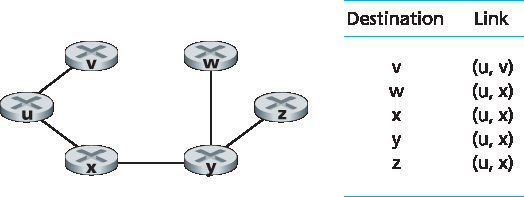
图 5.4 节点 u 的最小代价路径与转发表

该算法的计算复杂度是多少？也就是说，给定 n 个节点（不计入源节点），最坏情况下需要进行多少次计算才能找出从源到所有目的地的最小代价路径？第一次迭代需要在所有 n 个节点中查找具有最小代价的节点 w，第二次查找 n−1 个节点，第三次查找 n−2 个节点，依此类推。总的来说，所有迭代中查找的节点数为 n(n+1)/2，因此该 LS 算法的最坏时间复杂度为 n 的平方： $O (n^{2})$ 。（一种更高级的实现方式是使用称为堆的数据结构，在第 9 行中以对数时间而不是线性时间找出最小值，从而降低复杂度。）

在结束对 LS 算法的讨论前，让我们考虑一种可能出现的问题情形。图 5.5 显示了一个简单的网络拓扑，链路代价等于其所承载的负载，例如，反映经历的延迟。在此例中，链路代价是非对称的；即，只有当链路 (u, v) 在两个方向上承载相同流量时，才有 c(u, v) = c(v, u)。此例中，节点 z 发出一单位流量，目标为 w，节点 x 也发出一单位流量至 w，节点 y 注入 e 单位流量，也发往 w。初始路由如图 5.5(a) 所示，链路代价对应所承载的流量。

下一次运行 LS 算法时，节点 y 根据图 5.5(a) 中链路代价判断，顺时针路径代价为 1，而当前使用的逆时针路径代价为 1+e，因此 y 的最小代价路径改为顺时针方向。类似地，x 也判断出其最小代价路径变为顺时针方向，导致链路代价如图 5.5(b) 所示。再下一次运行 LS 算法时，x、y 和 z 都检测到逆时针方向路径代价为 0，因此都将流量切换到逆时针路径。再下一次运行时，它们又都将流量切回顺时针路径。

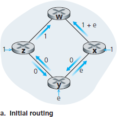
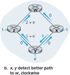
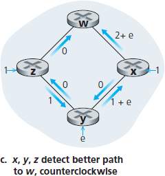
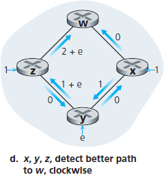
图 5.5 基于拥塞感知路由的震荡

如何避免这种震荡（这类震荡可能出现在任何使用拥塞或基于延迟的链路度量的算法中，而不仅限于 LS 算法）？一种解决方案是规定链路代价不得依赖于承载的流量——但这是不可接受的，因为路由的目标之一就是避开高度拥塞（例如高延迟）的链路。另一种解决方案是确保不是所有路由器同时运行 LS 算法。这似乎更合理，因为即使路由器以相同周期运行 LS 算法，但每个路由器的运行时刻应该不同。有趣的是，研究者发现互联网中的路由器之间可能会自同步 [Floyd Synchronization 1994]，即使初始时运行周期相同但时间点不同，最终这些算法执行实例会变得同步。避免这种自同步的一种方法是让每个路由器对其链路通告的发送时间进行随机化。

在学习完 LS 算法后，让我们转向当前实际中使用的另一主要路由算法 —— 距离向量路由算法。

原文

Recall that in a link-state algorithm, the network topology and all link costs are known, that is, available as input to the LS algorithm. In practice this is accomplished by having each node broadcast link-state packets to all other nodes in the network, with each link-state packet containing the identities and costs of its attached links. In practice (for example, with the Internet’s OSPF routing protocol, discussed in Section 5.3 ) this is often accomplished by a link-state broadcast algorithm :ref:[Perlman 1999] <Perlman 1999> . The result of the nodes’ broadcast is that all nodes have an identical and complete view of the network. Each node can then run the LS algorithm and compute the same set of least-cost paths as every other node.

The link-state routing algorithm we present below is known as Dijkstra’s algorithm, named after its inventor. A closely related algorithm is Prim’s algorithm; see [Cormen 2001] for a general discussion of graph algorithms. Dijkstra’s algorithm computes the least-cost path from one node (the source, which we will refer to as u) to all other nodes in the network. Dijkstra’s algorithm is iterative and has the property that after the kth iteration of the algorithm, the least-cost paths are known to k destination nodes, and among the least-cost paths to all destination nodes, these k paths will have the k smallest costs. Let us define the following notation:

D(v): cost of the least-cost path from the source node to destination v as of this iteration of the algorithm.
p(v): previous node (neighbor of v) along the current least-cost path from the source to v.
N′: subset of nodes; v is in N′ if the least-cost path from the source to v is definitively known.

The centralized routing algorithm consists of an initialization step followed by a loop. The number of times the loop is executed is equal to the number of nodes in the network. Upon termination, the algorithm will have calculated the shortest paths from the source node u to every other node in the network.

Link-State (LS) Algorithm for Source Node u#

 1  Initialization:
 2      N’ = {u}
 3      for all nodes v
 4          if v is a neighbor of u
 5              then D(v) = c(u, v)
 6          else D(v) = ∞
 7  Loop
 8      find w not in N’ such that D(w) is a minimum add w to N’
 9      update D(v) for each neighbor v of w and not in N’:
10
11          D(v) = min(D(v), D(w)+ c(w, v) )
12
13          /* new cost to v is either old cost to v or known least path cost to w plus cost from w to v */
14  until N’= N

As an example, let’s consider the network in Figure 5.3 and compute the least-cost paths from u to all possible destinations. A tabular summary of the algorithm’s computation is shown in Table 5.1, where each line in the table gives the values of the algorithm’s variables at the end of the iteration. Let’s consider the few first steps in detail.

In the initialization step, the currently known least-cost paths from u to its directly attached neighbors, v, x, and w, are initialized to 2, 1, and 5, respectively. Note in particular that the cost to w is set to 5 (even though we will soon see that a lesser-cost path does indeed exist) since this is the cost of the direct (one hop) link from u to w. The costs to y and z are set to infinity because they are not directly connected to u.

Table 5.1 Running the link-state algorithm on the network in Figure 5.3

step	N’	D(v), p(v)	D(w), p(w)	D(x), p(x)	D (y), p (y)	D (z), p (z)
0	u	2, u	5, u	1,u	∞	∞
1	ux	2, u	4, u		2, x	∞
2	uxy	2, u	3, y		2, x	4, y
3	uxyv		3, y			4, y
4	uxyvw					4, y
5	uxyvwz

In the first iteration, we look among those nodes not yet added to the set N′ and find that node with the least cost as of the end of the previous iteration. That node is x, with a cost of 1, and thus x is added to the set N′. Line 12 of the LS algorithm is then performed to update D(v) for all nodes v, yielding the results shown in the second line (Step 1) in Table 5.1. The cost of the path to v is unchanged. The cost of the path to w (which was 5 at the end of the initialization) through node x is found to have a cost of 4. Hence this lower-cost path is selected and w’s predecessor along the shortest path from u is set to x. Similarly, the cost to y (through x) is computed to be 2, and the table is updated accordingly.
In the second iteration, nodes v and y are found to have the least-cost paths (2), and we break the tie arbitrarily and add y to the set N′ so that N′ now contains u, x, and y. The cost to the remaining nodes not yet in N′, that is, nodes v, w, and z, are updated via line 12 of the LS algorithm, yielding the results shown in the third row in Table 5.1.
And so on …

When the LS algorithm terminates, we have, for each node, its predecessor along the least-cost path from the source node. For each predecessor, we also have its predecessor, and so in this manner we can construct the entire path from the source to all destinations. The forwarding table in a node, say node u, can then be constructed from this information by storing, for each destination, the next-hop node on the least-cost path from u to the destination. Figure 5.4 shows the resulting least-cost paths and forwarding table in u for the network in Figure 5.3.

Figure 5.4 Least cost path and forwarding table for node u

What is the computational complexity of this algorithm? That is, given n nodes (not counting the source), how much computation must be done in the worst case to find the least-cost paths from the source to all destinations? In the first iteration, we need to search through all n nodes to determine the node, w, not in N′ that has the minimum cost. In the second iteration, we need to check n−1 nodes to determine the minimum cost; in the third iteration n−2 nodes, and so on. Overall, the total number of nodes we need to search through over all the iterations is n(n+1)/2, and thus we say that the preceding implementation of the LS algorithm has worst-case complexity of order n squared: $O (n^{2})$ . (A more sophisticated implementation of this algorithm, using a data structure known as a heap, can find the minimum in line 9 in logarithmic rather than linear time, thus reducing the complexity.)

Before completing our discussion of the LS algorithm, let us consider a pathology that can arise. Figure 5.5 shows a simple network topology where link costs are equal to the load carried on the link, for example, reflecting the delay that would be experienced. In this example, link costs are not symmetric; that is, c(u, v) equals c(v, u) only if the load carried on both directions on the link (u, v) is the same. In this example, node z originates a unit of traffic destined for w, node x also originates a unit of traffic destined for w, and node y injects an amount of traffic equal to e, also destined for w. The initial routing is shown in Figure 5.5(a) with the link costs corresponding to the amount of traffic carried.

When the LS algorithm is next run, node y determines (based on the link costs shown in Figure 5.5(a) ) that the clockwise path to w has a cost of 1, while the counterclockwise path to w (which it had been using) has a cost of 1+e. Hence y’s least-cost path to w is now clockwise. Similarly, x determines that its new least-cost path to w is also clockwise, resulting in costs shown in Figure 5.5(b). When the LS algorithm is run next, nodes x, y, and z all detect a zero-cost path to w in the counterclockwise direction, and all route their traffic to the counterclockwise routes. The next time the LS algorithm is run, x, y, and z all then route their traffic to the clockwise routes.

Figure 5.5 Oscillations with congestion-sensitive routing

What can be done to prevent such oscillations (which can occur in any algorithm, not just an LS algorithm, that uses a congestion or delay-based link metric)? One solution would be to mandate that link costs not depend on the amount of traffic carried—an unacceptable solution since one goal of routing is to avoid highly congested (for example, high-delay) links. Another solution is to ensure that not all routers run the LS algorithm at the same time. This seems a more reasonable solution, since we would hope that even if routers ran the LS algorithm with the same periodicity, the execution instance of the algorithm would not be the same at each node. Interestingly, researchers have found that routers in the Internet can self-synchronize among themselves [Floyd Synchronization 1994]. That is, even though they initially execute the algorithm with the same period but at different instants of time, the algorithm execution instance can eventually become, and remain, synchronized at the routers. One way to avoid such self-synchronization is for each router to randomize the time it sends out a link advertisement.

Having studied the LS algorithm, let’s consider the other major routing algorithm that is used in practice today—the distance-vector routing algorithm.

5.2.2 距离向量（DV）路由算法#

5.2.2 The Distance-Vector (DV) Routing Algorithm

与使用全局信息的 LS 算法不同， 距离向量（DV） 算法是迭代的、异步的和分布式的。它是分布式的，因为每个节点从一个或多个直接相连的邻居接收信息，进行计算，然后将计算结果分发回其邻居。它是迭代的，因为该过程不断进行，直到邻居间不再交换信息。（有趣的是，该算法也是自终止的——没有停止计算的信号，算法自然停止。）该算法是异步的，因为它不要求所有节点必须同步运行。我们将看到，一个异步、迭代、自终止、分布式的算法比集中式算法更有趣也更好玩！

在介绍 DV 算法之前，讨论一个最小代价路径代价之间的重要关系会很有帮助。令 $d_{x} (y)$ 为节点 x 到节点 y 的最小代价路径代价。那么这些最小代价满足著名的 Bellman-Ford 方程，即：

(1)#

d_{x} (y) = m i n_{v} {c (x, v) + d_{v} (y)}

方程中的 $m i n_{v}$ 是对所有 x 的邻居 v 取最小。Bellman-Ford 方程相当直观。确实，从 x 到 v 后，如果再走 v 到 y 的最小代价路径，则路径代价为 $c (x, v) + d_{x} (y)$ 。由于必须先走到某个邻居 v，从 x 到 y 的最小代价就是对所有邻居 v 的 $c (x, v) + d_{x} (y)$ 取最小。

但对于怀疑该方程有效性的人，我们以图 5.3 中的源节点 u 和目的节点 z 来验证。源节点 u 有三个邻居：v、x 和 w。通过图中的各种路径可知 $d_{v} (z) = 5$ , $d_{x} (z) = 3$ , $d_{w} (z) = 3$ 。代入 (1)，以及 $c (u, v) = 2, c (u, x) = 1, c (u, w) = 5$ ，得到 $d_{u} (z) = m i n {2 + 5, 5 + 3, 1 + 3} = 4$ ，这显然正确，也正是 Dijkstra 算法给出的结果。这个快速验证应能消除你的疑虑。

Bellman-Ford 方程不仅是理论上的兴趣点，它有重要的实际意义：该方程的解为节点 x 的转发表条目提供依据。设 v* 为在 (1) 中取得最小值的邻居节点之一。那么，如果节点 x 想沿最小代价路径向节点 y 发送数据包，应先将包转发给邻居 v*。因此，节点 x 的转发表会指定 v* 作为目的节点 y 的下一跳路由器。Bellman-Ford 方程的另一个重要实际贡献是它表明了 DV 算法中邻居间通信的形式。

基本思路如下。每个节点 x 从 $D_{x} (y)$ 开始，这是它对从自身到网络中所有节点 y 的最小代价路径代价的估计。令 $D_{x} = [D_{x} (y) : y \in N]$ 为节点 x 的距离向量，即 x 到所有其他节点 y 的代价估计向量。在 DV 算法中，每个节点 x 维护以下路由信息：

对每个邻居 v，从 x 到直接邻居 v 的代价 $c (x, v)$
节点 x 的距离向量，即 $D_{x} = [D_{x} (y) : y \in N]$ ，包含 x 对所有目的节点 y 的代价估计
每个邻居的距离向量，即对 x 的每个邻居 v，有 $D_{v} = [D_{v} (y) : y \in N]$

在分布式异步算法中，每隔一段时间，每个节点将自己的距离向量发送给所有邻居。当节点 x 从某邻居 w 收到新的距离向量时，它保存 w 的距离向量，并用 Bellman-Ford 方程更新自己的距离向量：

$D_{x} (y) = m i n_{v} {c (x, v) + D_{v} (y)}$ 对每个节点 y ∈ N

如果经过此更新步骤后节点 x 的距离向量发生变化，节点 x 会将更新后的距离向量发送给所有邻居，邻居们也会相应更新自己的距离向量。令人惊奇的是，只要所有节点继续以异步方式交换距离向量，每个代价估计 Dx(y) 都会收敛到 dx(y)，即节点 x 到节点 y 的实际最小代价路径代价 [Bertsekas 1991]！

原文

Whereas the LS algorithm is an algorithm using global information, the distance-vector (DV) algorithm is iterative, asynchronous, and distributed. It is distributed in that each node receives some information from one or more of its directly attached neighbors, performs a calculation, and then distributes the results of its calculation back to its neighbors. It is iterative in that this process continues on until no more information is exchanged between neighbors. (Interestingly, the algorithm is also self-terminating—there is no signal that the computation should stop; it just stops.) The algorithm is asynchronous in that it does not require all of the nodes to operate in lockstep with each other. We’ll see that an asynchronous, iterative, self-terminating, distributed algorithm is much more interesting and fun than a centralized algorithm!

Before we present the DV algorithm, it will prove beneficial to discuss an important relationship that exists among the costs of the least-cost paths. Let dx(y) be the cost of the least-cost path from node x to node y. Then the least costs are related by the celebrated Bellman-Ford equation, namely,

dx(y)=minv{c(x,v)+dv(y)}, – (5.1)

where the minv in the equation is taken over all of x’s neighbors. The Bellman-Ford equation is rather intuitive. Indeed, after traveling from x to v, if we then take the least-cost path from v to y, the path cost will be c(x,v)+dv(y). Since we must begin by traveling to some neighbor v, the least cost from x to y is the minimum of c(x,v)+dv(y) taken over all neighbors v.

But for those who might be skeptical about the validity of the equation, let’s check it for source node u and destination node z in Figure 5.3. The source node u has three neighbors: nodes v, x, and w. By walking along various paths in the graph, it is easy to see that dv(z)=5, dx(z)=3, and dw(z)=3. Plugging these values into Equation 5.1, along with the costs c(u,v)=2, c(u,x)=1, and c(u,w)=5, gives du(z)=min{2+5,5+3,1+3}=4, which is obviously true and which is exactly what the Dijskstra algorithm gave us for the same network. This quick verification should help relieve any skepticism you may have.

The Bellman-Ford equation is not just an intellectual curiosity. It actually has significant practical importance: the solution to the Bellman-Ford equation provides the entries in node x’s forwarding table. To see this, let v* be any neighboring node that achieves the minimum in Equation 5.1. Then, if node x wants to send a packet to node y along a least-cost path, it should first forward the packet to node v*. Thus, node x’s forwarding table would specify node v* as the next-hop router for the ultimate destination y. Another important practical contribution of the Bellman-Ford equation is that it suggests the form of the neighbor-to-neighbor communication that will take place in the DV algorithm.

The basic idea is as follows. Each node x begins with Dx(y), an estimate of the cost of the least-cost path from itself to node y, for all nodes, y, in N. Let Dx=[Dx(y): y in N] be node x’s distance vector, which is the vector of cost estimates from x to all other nodes, y, in N. With the DV algorithm, each node x maintains the following routing information:

For each neighbor v, the cost c(x, v) from x to directly attached neighbor, v
Node x’s distance vector, that is, Dx=[Dx(y): y in N], containing x’s estimate of its cost to all destinations, y, in N
The distance vectors of each of its neighbors, that is, Dv=[Dv(y): y in N] for each neighbor v of x

In the distributed, asynchronous algorithm, from time to time, each node sends a copy of its distance vector to each of its neighbors. When a node x receives a new distance vector from any of its neighbors w, it saves w’s distance vector, and then uses the Bellman-Ford equation to update its own distance vector as follows:

Dx(y)=minv{c(x,v)+Dv(y)} for each node y in N

If node x’s distance vector has changed as a result of this update step, node x will then send its updated distance vector to each of its neighbors, which can in turn update their own distance vectors. Miraculously enough, as long as all the nodes continue to exchange their distance vectors in an asynchronous fashion, each cost estimate Dx(y) converges to dx(y), the actual cost of the least-cost path from node x to node y [Bertsekas 1991]!

距离向量（DV）算法#

Distance-Vector (DV) Algorithm

在每个节点 x：

 1 Initialization:
 2     for all destinations y in N:
 3         Dx(y) = c(x, y) /* 如果 y 不是邻居，则 c(x, y) = ∞ */
 4     for each neighbor w:
 5         Dw(y) = ?  /* 对所有目的地 y ∈ N */
 6     for each neighbor w:
 7         发送距离向量 Dx = [Dx(y): y ∈ N] 给 w
 8
 9     loop
10         wait（直到检测到某邻居 w 的链路代价变化 或
11                收到某邻居 w 的距离向量）
12         for each y in N:
13             Dx(y) = minv { c(x, v) + Dv(y) }
14
15         if Dx(y) changed for any destination y
16             发送更新后的距离向量 Dx = [Dx(y): y ∈ N] 给所有邻居
17
18     forever

在 DV 算法中，当节点 x 发现其直接相连链路代价发生变化，或者收到某邻居的距离向量更新时，会更新自己的距离向量。但要更新自己的转发表，对给定目的地 y，节点 x 需要知道的不是最短路径距离，而是下一跳路由器 v*(y)，即最短路径上目的地 y 的下一跳邻居。正如你所料，v*(y) 就是 DV 算法第 14 行取得最小值的邻居 v。（如果有多个邻居取得最小值，则 v*(y) 可以是任意一个最小邻居。）因此在算法第 13–14 行中，对于每个目的地 y，节点 x 还确定 v*(y) 并更新目的地 y 的转发表。

回想一下，LS 算法是集中式的，因为它要求每个节点先获得网络的完整地图，再运行 Dijkstra 算法。DV 算法则是去中心化的，不使用全局信息。节点仅知道到其直接邻居的链路代价和从邻居处获得的信息。每个节点等待任一邻居的更新（第 10–11 行），收到更新时计算新的距离向量（第 14 行），并将新距离向量分发给邻居（第 16–17 行）。DV 类算法广泛应用于许多实际路由协议，包括互联网的 RIP 和 BGP，ISO IDRP，Novell IPX，以及最初的 ARPAnet。

图 5.6 展示了 DV 算法在一个简单三节点网络中的操作。图中以同步方式展示算法过程，所有节点同时接收邻居的距离向量，计算新距离向量，并在距离向量发生变化时通知邻居。学习此例后，你应相信该算法同样能在异步环境下正确运行，节点的计算和更新随时发生。

图最左列显示三个节点的初始路由表。例如左上角的表是节点 x 的初始路由表。在一个路由表中，每行是一个距离向量——具体地，每个节点的路由表包含它自己的距离向量和每个邻居的距离向量。因此，节点 x 初始路由表的第一行为 $D_{x} = [D_{x} (x), D_{x} (y), D_{x} (z)] = [0, 2, 7]$ 。第二、三行分别是节点 y 和 z 最近接收的距离向量。由于初始化时节点 x 尚未收到来自 y 和 z 的距离向量，第二、三行条目初始化为无穷大。

初始化后，每个节点将其距离向量发送给两个邻居，见图 5.6 中从第一列表格指向第二列表格的箭头。例如节点 x 将 $D_{x} = [0, 2, 7]$ 发送给节点 y 和 z。收到更新后，每个节点重新计算自己的距离向量。例如，节点 x 计算：

\begin{array}{r} \begin{aligned} D_{x} (x) = 0 \\ D_{x} (y) = m i n {c (x, y) + D_{y} (y), c (x, z) + D_{z} (y)} = m i n {2 + 0, 7 + 1} = 2 \\ D_{x} (z) = m i n {c (x, y) + D_{y} (z), c (x, z) + D_{z} (z)} = m i n {2 + 1, 7 + 0} = 3 \end{aligned} \end{array}

因此第二列显示每个节点的新距离向量以及从邻居刚收到的距离向量。注意节点 x 对节点 z 的最小代价估计 $D_{x} (z)$ 从 7 改变为 3。且节点 x 的邻居 y 在算法第 14 行中取得最小值，因此此阶段在节点 x 处, $v * (y) = y$ , $v * (z) = y$ 。

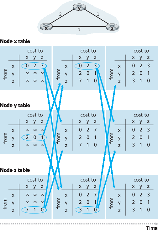
图 5.6 距离向量（DV）算法运行示意

节点重新计算距离向量后，再将更新的距离向量发送给邻居（如果有变化）。见图 5.6 中第二列指向第三列表的箭头。注意只有节点 x 和 z 发送了更新，节点 y 的距离向量未变，因此未发送更新。收到更新后，节点再次重新计算距离向量并更新路由表，见第三列。

邻居发送更新距离向量、节点重新计算路由表条目、通知邻居最小路径代价变化的过程不断进行，直到不再有更新消息发送。此时算法进入静止状态，即所有节点都在第 10–11 行等待。算法将保持静止状态，直到链路代价发生变化，如下文所述。

原文

At each node, x:

 1 Initialization:
 2     for all destinations y in N:
 3         Dx(y)= c(x, y)/* if y is not a neighbor then c(x, y)= ∞ */
 4     for each neighbor w
 5         Dw(y) = ? for all destinations y in N
 6     for each neighbor w
 7         send distance vector Dx = [Dx(y): y in N] to w
 8
 9     loop
10         wait (until I see a link cost change to some neighbor w or
11                    until I receive a distance vector from some neighbor w)
12         for each y in N:
13             Dx(y) = minv{c(x, v) + Dv(y)}
14
15         if Dx(y) changed for any destination y
16             send distance vector Dx = [Dx(y): y in N] to all neighbors 18
17
18     forever

In the DV algorithm, a node x updates its distance-vector estimate when it either sees a cost change in one of its directly attached links or receives a distance-vector update from some neighbor. But to update its own forwarding table for a given destination y, what node x really needs to know is not the shortest-path distance to y but instead the neighboring node v*(y) that is the next-hop router along the shortest path to y. As you might expect, the next-hop router v*(y) is the neighbor v that achieves the minimum in Line 14 of the DV algorithm. (If there are multiple neighbors v that achieve the minimum, then v*(y) can be any of the minimizing neighbors.) Thus, in Lines 13–14, for each destination y, node x also determines v*(y) and updates its forwarding table for destination y.

Recall that the LS algorithm is a centralized algorithm in the sense that it requires each node to first obtain a complete map of the network before running the Dijkstra algorithm. The DV algorithm is decentralized and does not use such global information. Indeed, the only information a node will have is the costs of the links to its directly attached neighbors and information it receives from these neighbors. Each node waits for an update from any neighbor (Lines 10–11), calculates its new distance vector when receiving an update (Line 14), and distributes its new distance vector to its neighbors (Lines 16–17). DV-like algorithms are used in many routing protocols in practice, including the Internet’s RIP and BGP, ISO IDRP, Novell IPX, and the original ARPAnet.

Figure 5.6 illustrates the operation of the DV algorithm for the simple three-node network shown at the top of the figure. The operation of the algorithm is illustrated in a synchronous manner, where all nodes simultaneously receive distance vectors from their neighbors, compute their new distance vectors, and inform their neighbors if their distance vectors have changed. After studying this example, you should convince yourself that the algorithm operates correctly in an asynchronous manner as well, with node computations and update generation/reception occurring at any time.

The leftmost column of the figure displays three initial routing tables for each of the three nodes. For example, the table in the upper-left corner is node x’s initial routing table. Within a specific routing table, each row is a distance vector— specifically, each node’s routing table includes its own distance vector and that of each of its neighbors. Thus, the first row in node x’s initial routing table is Dx=[Dx(x),Dx(y),Dx(z)]=[0,2,7]. The second and third rows in this table are the most recently received distance vectors from nodes y and z, respectively. Because at initialization node x has not received anything from node y or z, the entries in the second and third rows are initialized to infinity.

After initialization, each node sends its distance vector to each of its two neighbors. This is illustrated in Figure 5.6 by the arrows from the first column of tables to the second column of tables. For example, node x sends its distance vector Dx = [0, 2, 7] to both nodes y and z. After receiving the updates, each node recomputes its own distance vector. For example, node x computes

Dx(x)=0Dx(y)=min{c(x,y)+Dy(y),c(x,z)+Dz(y)}=min{2+0, 7+1}=2Dx(z)=min{c(x,y)+Dy(z),c(x,z)+Dz(z)}=min{2+1,7+0}=3

The second column therefore displays, for each node, the node’s new distance vector along with distance vectors just received from its neighbors. Note, for example, that node x’s estimate for the least cost to node z, Dx(z), has changed from 7 to 3. Also note that for node x, neighboring node y achieves the minimum in line 14 of the DV algorithm; thus at this stage of the algorithm, we have at node x that v*(y)=y and v*(z)=y.

Figure 5.6 Distance-vector (DV) algorithm in operation

After the nodes recompute their distance vectors, they again send their updated distance vectors to their neighbors (if there has been a change). This is illustrated in Figure 5.6 by the arrows from the second column of tables to the third column of tables. Note that only nodes x and z send updates: node y’s distance vector didn’t change so node y doesn’t send an update. After receiving the updates, the nodes then recompute their distance vectors and update their routing tables, which are shown in the third column.

The process of receiving updated distance vectors from neighbors, recomputing routing table entries, and informing neighbors of changed costs of the least-cost path to a destination continues until no update messages are sent. At this point, since no update messages are sent, no further routing table calculations will occur and the algorithm will enter a quiescent state; that is, all nodes will be performing the wait in Lines 10–11 of the DV algorithm. The algorithm remains in the quiescent state until a link cost changes, as discussed next.

距离向量算法：链路代价变化与链路故障#

Distance-Vector Algorithm: Link-Cost Changes and Link Failure

当运行 DV 算法的节点检测到其到邻居的链路代价变化（第 10–11 行），它会更新距离向量（第 13–14 行），并在最小路径代价变化时通知邻居（第 16–17 行）。图 5.7(a) 描述了 y 到 x 的链路代价由 4 变为 1 的场景。我们只关注 y 和 z 的距离表条目（目的地 x）。DV 算法导致以下事件序列发生：

时间 t0，y 发现链路代价变化（从 4 变为 1），更新距离向量，并通知邻居因为其距离向量已变。
时间 t1，z 收到 y 的更新，更新路由表。其到 x 的最小代价由 5 降至 2，并将新距离向量发送给邻居。
时间 t2，y 收到 z 的更新，更新路由表。y 的最小代价未变，因此不向 z 发送消息。算法进入静止状态。

因此，DV 算法仅需两次迭代即可进入静止状态。x 和 y 之间链路代价降低的好消息迅速传播到网络。

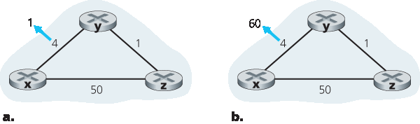
图 5.7 链路代价变化

接下来考虑链路代价上升的情况。假设 x 和 y 之间链路代价从 4 上升到 60，如图 5.7(b) 所示。

链路代价变化前， $D_{y} (x) = 4$ ， $D_{y} (z) = 1$ ， $D_{z} (y) = 1$ ， $D_{z} (x) = 5$ 。时间 t0，y 发现链路代价变化（4 变 60）。y 计算其到 x 的最小代价：

$D_{y} (x) = m i n {c (y, x) + D_{x} (x), c (y, z) + D_{z} (x)} = m i n {60 + 0, 1 + 5} = 6$

当然从网络全局视角看，途经 z 的新代价是错误的。但 y 只知道直接到 x 的代价是 60，且 z 最后告诉 y 到 x 的代价是 5。所以 y 现在会选择通过 z 到达 x，期望 z 能以代价 5 到达 x。时间 t1 时形成了 路由环路 ——为到达 x，y 通过 z 路由，z 又通过 y 路由。路由环路类似黑洞，发往 x 的数据包在 y 和 z 间永远循环（直到转发表改变）。
由于 y 计算出到 x 的新最小代价，它在 t1 时通知 z 自己的新距离向量。
t1 后不久，z 收到 y 的新距离向量，得知 y 到 x 的最小代价为 6。z 知道到 y 的代价是 1，因此计算新的最小代价：

$D_{z} (x) = m i n {50 + 0, 1 + 6} = 7$

由于 Dz(x) 增加，z 在 t2 通知 y 新距离向量。
类似地，y 收到 z 更新后计算 $D_{y} (x) = 8$ ，通知 z；z 计算 $D_{z} (x) = 9$ ，通知 y，如此循环。

该过程将持续多久？你应能确信该环路将持续 44 次迭代（y 和 z 之间的消息交换）——直到 z 最终计算出其通过 y 到 x 的路径代价超过 50。此时 z （终于！）认定其最小代价路径是直接连接到 x，y 也会通过 z 路由到 x。链路代价上升的坏消息传播非常缓慢！如果链路代价 $c (y, x)$ 从 4 变为 10000，而 $c (z, x)$ 为 9999，会怎样？正因为此类情况，我们称之为计数到无穷（count-to-infinity）问题。

原文

When a node running the DV algorithm detects a change in the link cost from itself to a neighbor (Lines 10–11), it updates its distance vector (Lines 13–14) and, if there’s a change in the cost of the least-cost path, informs its neighbors (Lines 16–17) of its new distance vector. Figure 5.7(a) illustrates a scenario where the link cost from y to x changes from 4 to 1. We focus here only on y’ and z’s distance table entries to destination x. The DV algorithm causes the following sequence of events to occur:

At time t0, y detects the link-cost change (the cost has changed from 4 to 1), updates its distance vector, and informs its neighbors of this change since its distance vector has changed.
At time t1, z receives the update from y and updates its table. It computes a new least cost to x (it has decreased from a cost of 5 to a cost of 2) and sends its new distance vector to its neighbors.
At time t2, y receives z’s update and updates its distance table. y’s least costs do not change and hence y does not send any message to z. The algorithm comes to a quiescent state.

Thus, only two iterations are required for the DV algorithm to reach a quiescent state. The good news about the decreased cost between x and y has propagated quickly through the network.

Figure 5.7 Changes in link cost

Let’s now consider what can happen when a link cost increases. Suppose that the link cost between x and y increases from 4 to 60, as shown in Figure 5.7(b).

Before the link cost changes, Dy(x)=4, Dy(z)=1, Dz(y)=1, and Dz(x)=5. At time t0, y detects the link-cost change (the cost has changed from 4 to 60). y computes its new minimum-cost path to x to have a cost of

Dy(x)=min{c(y,x)+Dx(x), c(y,z)+Dz(x)}=min{60+0,1+5}=6

Of course, with our global view of the network, we can see that this new cost via z is wrong. But the only information node y has is that its direct cost to x is 60 and that z has last told y that z could get to x with a cost of 5. So in order to get to x, y would now route through z, fully expecting that z will be able to get to x with a cost of 5. As of t1 we have a routing loop—in order to get to x, y routes through z, and z routes through y. A routing loop is like a black hole—a packet destined for x arriving at y or z as of t1 will bounce back and forth between these two nodes forever (or until the forwarding tables are changed).
Since node y has computed a new minimum cost to x, it informs z of its new distance vector at time $t_{1}$ .
Sometime after t1, z receives y’s new distance vector, which indicates that y’s minimum cost to x is 6. z knows it can get to y with a cost of 1 and hence computes a new least cost to x of Dz(x)=min{50+0,1+6}=7. Since z’s least cost to x has increased, it then informs y of its new distance vector at $t_{2}$ .
In a similar manner, after receiving z’s new distance vector, y determines Dy(x)=8 and sends z its distance vector. z then determines Dz(x)=9 and sends y its distance vector, and so on.

How long will the process continue? You should convince yourself that the loop will persist for 44 iterations (message exchanges between y and z)—until z eventually computes the cost of its path via y to be greater than 50. At this point, z will (finally!) determine that its least-cost path to x is via its direct connection to x. y will then route to x via z. The result of the bad news about the increase in link cost has indeed traveled slowly! What would have happened if the link cost c(y, x) had changed from 4 to 10,000 and the cost c(z, x) had been 9,999? Because of such scenarios, the problem we have seen is sometimes referred to as the count-to-infinity problem.

距离向量算法：添加毒性逆转#

Distance-Vector Algorithm: Adding Poisoned Reverse

前面描述的特定环路场景可以通过一种称为 毒性逆转（poisoned reverse） 的技术来避免。其思想很简单——如果 z 通过 y 到达目的地 x，那么 z 会向 y 宣称其到 x 的距离为无穷大，即 z 会告诉 y: $D_{z} (x) = \infty$ （即使 z 实际上知道 $D_{z} (x) = 5$ ）。只要 z 仍然通过 y 路由到 x，它就会继续对 y 撒这个善意的谎言。因为 y 认为 z 无法到达 x，只要 z 继续通过 y 路由到 x（并谎称不是），y 就永远不会试图通过 z 到达 x。

现在我们来看毒性逆转如何解决我们先前在图 5.5(b) 中遇到的特定环路问题。由于毒性逆转，y 的距离表显示 $D_{z} (x) = \infty$ 。当 (x, y) 链路的代价在时间 t0 从 4 变为 60 时，y 更新其路由表并继续直接路由到 x，尽管代价更高为 60，同时通知 z 它到 x 的新代价，即 $D_{y} (x) = 60$ 。在 t1 接收到更新后，z 立即将其到 x 的路由切换为直接通过 (z, x) 链路，代价为 50。由于这是到 x 的一条新最小代价路径，且路径不再经过 y，z 现在在 t2 通知 y: $D_{z} (x) = 50$ 。收到 z 的更新后，y 将其距离表更新为 $D_{y} (x) = 51$ 。同时，因为 z 现在处于 y 到 x 的最小代价路径上，y 在 t3 告诉 z： $D_{y} (x) = \infty$ （即使 y 实际知道 $D_{y} (x) = 51$ ），以毒性逆转方式屏蔽从 z 到 x 的反向路径。

毒性逆转是否能解决通用的计数到无穷问题？不能。你应能确信，对于包含三个或更多节点的环路（而不是仅仅两个相邻节点），毒性逆转技术无法检测到。

原文

The specific looping scenario just described can be avoided using a technique known as poisoned reverse. The idea is simple—if z routes through y to get to destination x, then z will advertise to y that its distance to x is infinity, that is, z will advertise to y that Dz(x)=∞ (even though z knows Dz(x)=5 in truth). z will continue telling this little white lie to y as long as it routes to x via y. Since y believes that z has no path to x, y will never attempt to route to x via z, as long as z continues to route to x via y (and lies about doing so).

Let’s now see how poisoned reverse solves the particular looping problem we encountered before in Figure 5.5(b). As a result of the poisoned reverse, y’s distance table indicates Dz(x)=∞. When the cost of the (x, y) link changes from 4 to 60 at time t0, y updates its table and continues to route directly to x, albeit at a higher cost of 60, and informs z of its new cost to x, that is, Dy(x)=60. After receiving the update at t1, z immediately shifts its route to x to be via the direct (z, x) link at a cost of 50. Since this is a new least-cost path to x, and since the path no longer passes through y, z now informs y that Dz(x)=50 at t2. After receiving the update from z, y updates its distance table with Dy(x)=51. Also, since z is now on y’s least- cost path to x, y poisons the reverse path from z to x by informing z at time t3 that Dy(x)=∞ (even though y knows that Dy(x)=51 in truth).

Does poisoned reverse solve the general count-to-infinity problem? It does not. You should convince yourself that loops involving three or more nodes (rather than simply two immediately neighboring nodes) will not be detected by the poisoned reverse technique.

LS 和 DV 路由算法的比较#

A Comparison of LS and DV Routing Algorithm

DV 和 LS 算法在计算路由的方式上采取互补的策略。在 DV 算法中，每个节点只与其直接连接的邻居通信，但会向邻居提供从自己到网络中所有节点（它已知的）的最小代价估计。而 LS 算法则要求全局信息。因此，在实现中，例如在图 4.2 和图 5.1 中，每个节点需通过广播与所有其他节点通信，但它只报告自己直接连接链路的代价。我们以对一些特性的快速比较来结束对 LS 和 DV 算法的研究。回忆一下，N 是节点（路由器）集合，E 是边（链路）集合。

消息复杂度。我们已看到，LS 要求每个节点知道网络中每条链路的代价。这需要发送 $O (| N | | E |)$ 条消息。此外，每当链路代价发生变化时，新的链路代价必须发送给所有节点。DV 算法则在每次迭代中要求直接连接的邻居之间交换消息。我们已经看到，算法收敛所需的时间可能依赖于许多因素。当链路代价变化时，只有当新链路代价导致该链路上的某个节点的最小代价路径变化时，DV 算法才会传播该变化的结果。
收敛速度。我们已看到我们的 LS 实现是一个 $O (| N |^{2})$ 的算法，需要 $O (| N | | E |)$ 条消息。DV 算法可能收敛缓慢，并且在收敛过程中可能产生路由环路。DV 还受到计数到无穷问题的困扰。
鲁棒性。如果某个路由器发生故障、表现异常或被破坏，会发生什么？在 LS 中，路由器可以广播其某条连接链路的错误代价（但不能广播其他链路）。一个节点也可能破坏或丢弃它作为 LS 广播一部分接收到的任何分组。但 LS 节点仅计算自己的转发表；其他节点为自己执行类似的计算。这意味着 LS 下的路由计算是相对独立的，从而提供了一定程度的鲁棒性。在 DV 中，一个节点可以向任意或所有目的地发布错误的最小代价路径。（确实，在 1997 年，一个小型 ISP 中故障的路由器向国家主干网路由器提供了错误的路由信息。这导致其他路由器将大量流量发送到该故障路由器，并使互联网的大部分区域长达数小时无法连接 [Neumann 1997]。）更普遍地说，我们注意到，在每次迭代中，DV 中一个节点的计算会传递给其邻居，然后在下一轮迭代中间接传递给邻居的邻居。从这个意义上说，DV 中一个错误节点的计算可能扩散到整个网络。

最终，没有哪种算法明显优于另一种；事实上，两种算法都在互联网中被使用。

原文

The DV and LS algorithms take complementary approaches toward computing routing. In the DV algorithm, each node talks to only its directly connected neighbors, but it provides its neighbors with least- cost estimates from itself to all the nodes (that it knows about) in the network. The LS algorithm requires global information. Consequently, when implemented in each and every router, e.g., as in Figure 4.2 and 5.1, each node would need to communicate with all other nodes (via broadcast), but it tells them only the costs of its directly connected links. Let’s conclude our study of LS and DV algorithms with a quick comparison of some of their attributes. Recall that N is the set of nodes (routers) and E is the set of edges (links).

Message complexity. We have seen that LS requires each node to know the cost of each link in the network. This requires $O (| N | | E |)$ messages to be sent. Also, whenever a link cost changes, the new link cost must be sent to all nodes. The DV algorithm requires message exchanges between directly connected neighbors at each iteration. We have seen that the time needed for the algorithm to converge can depend on many factors. When link costs change, the DV algorithm will propagate the results of the changed link cost only if the new link cost results in a changed least-cost path for one of the nodes attached to that link.
Speed of convergence. We have seen that our implementation of LS is an $O (| N |^{2})$ algorithm requiring $O (| N | | E |)$ messages. The DV algorithm can converge slowly and can have routing loops while the algorithm is converging. DV also suffers from the count-to-infinity problem.
Robustness. What can happen if a router fails, misbehaves, or is sabotaged? Under LS, a router could broadcast an incorrect cost for one of its attached links (but no others). A node could also corrupt or drop any packets it received as part of an LS broadcast. But an LS node is computing only its own forwarding tables; other nodes are performing similar calculations for themselves. This means route calculations are somewhat separated under LS, providing a degree of robustness. Under DV, a node can advertise incorrect least-cost paths to any or all destinations. (Indeed, in 1997, a malfunctioning router in a small ISP provided national backbone routers with erroneous routing information. This caused other routers to flood the malfunctioning router with traffic and caused large portions of the Internet to become disconnected for up to several hours [Neumann 1997].) More generally, we note that, at each iteration, a node’s calculation in DV is passed on to its neighbor and then indirectly to its neighbor’s neighbor on the next iteration. In this sense, an incorrect node calculation can be diffused through the entire network under DV.

In the end, neither algorithm is an obvious winner over the other; indeed, both algorithms are used in the Internet.

5.2 路由算法

目录