6.2 错误检测与纠正技术#
6.2 Error-Detection and -Correction Techniques
在上一节中,我们提到, 比特级的错误检测与纠正 ——即检测和纠正从一个节点发送到另一个物理相邻节点的链路层帧中的比特损坏——是链路层通常提供的两项服务。在 第3章 中我们也看到,错误检测与纠正服务常常在传输层中提供。本节中,我们将考察一些最简单的用于检测(在某些情况下也能纠正)比特错误的技术。全面探讨该主题的理论与实现本身就是许多教材的内容(例如 [Schwartz 1980] 或 [Bertsekas 1991]),因此我们这里只做简要介绍。我们的目标是对错误检测与纠正技术所能提供的能力建立直观理解,并了解几个简单技术在链路层中的实际工作原理和使用方式。
图 6.3 展示了我们的研究场景。在发送节点,待保护的数据 D 会被附加上错误检测与纠正比特(EDC)。通常,待保护的数据不仅包括从网络层下传到链路层用于传输的数据报,也包括链路级地址信息、序列号以及帧头中的其他字段。 D 和 EDC 都会一起被打包进链路层帧发送到接收节点。在接收节点,会接收到一组比特序列 D' 和 EDC'。注意,由于传输中的比特翻转, D' 和 EDC' 可能与原始的 D 和 EDC 不同。
接收方的挑战是,仅凭接收到的 D‘ 和 EDC',来判断 D' 是否等于原始的 D。在 图 6.3 中对接收方决策的表述非常关键(我们问的是是否检测到错误,而不是是否发生了错误!)。错误检测与纠正技术可以让接收方有时(但并非总是)检测到比特错误的发生。即使使用了错误检测比特,仍然可能存在 未检测到的比特错误 ,即接收方无法察觉接收到的信息中包含比特错误。因此,接收方可能会将一个损坏的数据报递交给网络层,或者没能察觉帧头中的某个字段已经损坏。因此,我们希望选择一种能尽可能降低此类错误概率的错误检测机制。通常,越复杂的错误检测与纠正技术(即未检测到错误的概率越小)所带来的开销也越大——需要更多的计算资源来计算和传输更多的检测与纠正比特。
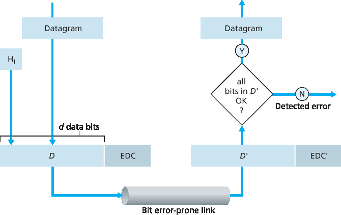
图 6.3 错误检测与纠正场景
现在我们来看看三种数据传输中错误检测技术——奇偶校验(用于说明错误检测与纠正的基本概念)、校验和方法(通常用于传输层)以及循环冗余校验(CRC,通常用于链路层和适配器中)。
In the previous section, we noted that bit-level error detection and correction—detecting and correcting the corruption of bits in a link-layer frame sent from one node to another physically connected neighboring node—are two services often provided by the link layer. We saw in Chapter 3 that error- detection and -correction services are also often offered at the transport layer as well. In this section, we’ll examine a few of the simplest techniques that can be used to detect and, in some cases, correct such bit errors. A full treatment of the theory and implementation of this topic is itself the topic of many textbooks (for example, [Schwartz 1980] or [Bertsekas 1991]), and our treatment here is necessarily brief. Our goal here is to develop an intuitive feel for the capabilities that error-detection and -correction techniques provide and to see how a few simple techniques work and are used in practice in the link layer.
Figure 6.3 illustrates the setting for our study. At the sending node, data, D, to be protected against bit errors is augmented with error-detection and -correction bits (EDC). Typically, the data to be protected includes not only the datagram passed down from the network layer for transmission across the link, but also link-level addressing information, sequence numbers, and other fields in the link frame header. Both D and EDC are sent to the receiving node in a link-level frame. At the receiving node, a sequence of bits, D′ and EDC′ is received. Note that D′ and EDC′ may differ from the original D and EDC as a result of in-transit bit flips.
The receiver’s challenge is to determine whether or not D′ is the same as the original D, given that it has only received D′ and EDC′. The exact wording of the receiver’s decision in Figure 6.3 (we ask whether an error is detected, not whether an error has occurred!) is important. Error-detection and -correction techniques allow the receiver to sometimes, but not always, detect that bit errors have occurred. Even with the use of error-detection bits there still may be undetected bit errors; that is, the receiver may be unaware that the received information contains bit errors. As a consequence, the receiver might deliver a corrupted datagram to the network layer, or be unaware that the contents of a field in the frame’s header has been corrupted. We thus want to choose an error- detection scheme that keeps the probability of such occurrences small. Generally, more sophisticated error-detection and-correction techniques (that is, those that have a smaller probability of allowing undetected bit errors) incur a larger overhead—more computation is needed to compute and transmit a larger number of error-detection and -correction bits.
Figure 6.3 Error-detection and -correction scenario
Let’s now examine three techniques for detecting errors in the transmitted data—parity checks (to illustrate the basic ideas behind error detection and correction), checksumming methods (which are more typically used in the transport layer), and cyclic redundancy checks (which are more typically used in the link layer in an adapter).
6.2.1 奇偶校验#
6.2.1 Parity Checks
最简单的错误检测形式可能是使用单个 奇偶校验位。假设要发送的信息 D 如 图 6.4 所示,共有 d 个比特。在偶校验方案中,发送方只需添加一个额外比特,并设置其值,使得 d+1 个比特(原始数据加上奇偶校验位)中 1 的个数为偶数。在奇校验方案中,奇偶校验位的值应使得 1 的个数为奇数。图 6.4 展示了一个偶校验的方案,其中单个位的奇偶校验被保存在一个单独的字段中。
当使用单个奇偶校验位时,接收方的操作也很简单。接收方只需统计收到的 d+1 个比特中 1 的数量。如果使用偶校验方案时发现有奇数个 1,则说明至少发生了一个比特错误。更准确地说,是发生了奇数个比特错误。
但如果发生的是偶数个比特错误会怎样?你可以验证一下,这种情况将导致错误未被检测到。如果比特错误概率较小,并且可以假设错误在各比特间是独立发生的,那么一个分组中发生多个比特错误的概率将非常小。在这种情况下,使用单个奇偶校验位可能已足够。然而,实际测量表明,错误通常并非独立发生,而是集中成“突发错误”。在突发错误条件下,单个位奇偶校验保护的帧中未检测到错误的概率可能高达 50% [Spragins 1991]。显然,需要一种更健壮的错误检测方案(幸运的是,实践中确实使用了更健壮的方案!)。但在探讨实际使用的错误检测方案之前,我们先来看单个位奇偶校验的一种简单推广,它将帮助我们理解错误纠正技术。
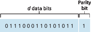
图 6.4 单个位偶校验
图 6.5 展示了单个位奇偶校验方案的二维推广形式。这里, d 个比特被划分为 i 行 j 列。每一行和每一列都计算一个奇偶校验值。最终产生的 i+j+1 个奇偶校验位构成链路层帧的错误检测比特。
假设现在在原始 d 个比特中发生了一个比特错误。在这种 二维奇偶校验 方案中,包含错误比特的行和列的奇偶校验都会出错。因此,接收方不仅可以检测到发生了单个比特错误,还可以通过错误行和列的索引,定位出损坏的比特并纠正错误!图 6.5 展示了一个例子:位置 (2,2) 的值为 1 的比特被翻转为0——这是一个接收方可以检测并纠正的错误。虽然我们主要关注的是原始的 d 个比特,但即使奇偶校验位本身发生错误,也可以被检测并纠正。二维奇偶校验还可以检测(但不能纠正)任意两个比特的组合错误。有关二维奇偶校验方案的其他特性将在本章末尾的习题中探讨。
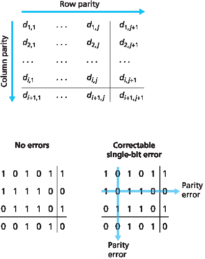
图 6.5 二维偶校验
接收方既能检测又能纠正错误的能力称为 前向纠错(FEC)。这些技术广泛应用于音频存储与播放设备,如音频 CD。在网络环境中,FEC 技术可以独立使用,也可以与类似于我们在 第3章 中讨论的链路层 ARQ 技术结合使用。FEC 技术的价值在于它能减少发送方所需的重传次数。更重要的是,它允许接收方即时纠正错误,避免了等待往返传播延迟以接收 NAK 包及重传包返回的过程——这对实时网络应用 [Rubenstein 1998] 或传播延迟长的链路(如深空链路)来说尤为重要。研究 FEC 在错误控制协议中应用的相关文献包括 [Biersack 1992;Nonnenmacher 1998;Byers 1998;Shacham 1990]。
Perhaps the simplest form of error detection is the use of a single parity bit. Suppose that the information to be sent, D in Figure 6.4, has d bits. In an even parity scheme, the sender simply includes one additional bit and chooses its value such that the total number of 1s in the d+1 bits (the original information plus a parity bit) is even. For odd parity schemes, the parity bit value is chosen such that there is an odd number of 1s. Figure 6.4 illustrates an even parity scheme, with the single parity bit being stored in a separate field.
Receiver operation is also simple with a single parity bit. The receiver need only count the number of 1s in the received d+1 bits. If an odd number of 1-valued bits are found with an even parity scheme, the receiver knows that at least one bit error has occurred. More precisely, it knows that some odd number of bit errors have occurred.
But what happens if an even number of bit errors occur? You should convince yourself that this would result in an undetected error. If the probability of bit errors is small and errors can be assumed to occur independently from one bit to the next, the probability of multiple bit errors in a packet would be extremely small. In this case, a single parity bit might suffice. However, measurements have shown that, rather than occurring independently, errors are often clustered together in “bursts.” Under burst error conditions, the probability of undetected errors in a frame protected by single-bit parity can approach 50 percent [Spragins 1991]. Clearly, a more robust error-detection scheme is needed (and, fortunately, is used in practice!). But before examining error-detection schemes that are used in practice, let’s consider a simple generalization of one-bit parity that will provide us with insight into error-correction techniques.
Figure 6.4 One-bit even parity
Figure 6.5 shows a two-dimensional generalization of the single-bit parity scheme. Here, the d bits in D are divided into i rows and j columns. A parity value is computed for each row and for each column. The resulting i+j+1 parity bits comprise the link-layer frame’s error-detection bits.
Suppose now that a single bit error occurs in the original d bits of information. With this two-dimensional parity scheme, the parity of both the column and the row containing the flipped bit will be in error. The receiver can thus not only detect the fact that a single bit error has occurred, but can use the column and row indices of the column and row with parity errors to actually identify the bit that was corrupted and correct that error! Figure 6.5 shows an example in which the 1-valued bit in position (2,2) is corrupted and switched to a 0—an error that is both detectable and correctable at the receiver. Although our discussion has focused on the original d bits of information, a single error in the parity bits themselves is also detectable and correctable. Two-dimensional parity can also detect (but not correct!) any combination of two errors in a packet. Other properties of the two-dimensional parity scheme are explored in the problems at the end of the chapter.
Figure 6.5 Two-dimensional even parity
The ability of the receiver to both detect and correct errors is known as forward error correction (FEC). These techniques are commonly used in audio storage and playback devices such as audio CDs. In a network setting, FEC techniques can be used by themselves, or in conjunction with link-layer ARQ techniques similar to those we examined in Chapter 3. FEC techniques are valuable because they can decrease the number of sender retransmissions required. Perhaps more important, they allow for immediate correction of errors at the receiver. This avoids having to wait for the round-trip propagation delay needed for the sender to receive a NAK packet and for the retransmitted packet to propagate back to the receiver—a potentially important advantage for real-time network applications [Rubenstein 1998] or links (such as deep-space links) with long propagation delays. Research examining the use of FEC in error-control protocols includes [Biersack 1992; Nonnenmacher 1998; Byers 1998; Shacham 1990].
6.2.2 校验和方法#
6.2.2 Checksumming Methods
在校验和技术中, 图 6.4 中的 d 位数据被视为一组 k 位整数序列。一种简单的校验和方法就是将这些 k 位整数相加,并使用所得总和作为错误检测比特。Internet 校验和就是基于该方法实现的——数据按字节划分为 16 位整数并求和。其 1 的补码即构成携带在段头中的 Internet 校验和。如 第3.3节 所述,接收方通过计算接收到的数据(包括校验和)的总和的 1 的补码,并检查结果是否全为 1 来验证校验和。如果存在任何 0,则说明发生了错误。 RFC 1071 中详细讨论了 Internet 校验和算法及其实现。在 TCP 和 UDP 协议中,Internet 校验和计算覆盖所有字段(包括头部和数据字段)。而在 IP 协议中,校验和只覆盖 IP 头部(因为 UDP 或 TCP 段有自己的校验和)。在其他协议中,例如 XTP [Strayer 1992],会分别计算头部校验和与整个数据包的校验和。
校验和方法的报文开销相对较小。例如,在 TCP 和 UDP 中,校验和仅使用 16 位。然而,与接下来讨论的循环冗余校验(CRC)相比,它们提供的错误保护能力相对较弱。此时一个自然的问题是,为什么传输层使用校验和而链路层使用 CRC?回想一下,传输层通常作为主机操作系统的一部分由软件实现。因为传输层错误检测是由软件实现的,因此使用像校验和这样简单快速的检测方法显得尤为重要。而链路层的错误检测则由适配器中的专用硬件实现,能够快速完成更复杂的 CRC 运算。Feldmeier [Feldmeier 1995] 提出了快速实现加权校验和代码、CRC(见下文)及其他代码的软件技术。
In checksumming techniques, the d bits of data in Figure 6.4 are treated as a sequence of k-bit integers. One simple checksumming method is to simply sum these k-bit integers and use the resulting sum as the error-detection bits. The Internet checksum is based on this approach—bytes of data are treated as 16-bit integers and summed. The 1s complement of this sum then forms the Internet checksum that is carried in the segment header. As discussed in Section 3.3, the receiver checks the checksum by taking the 1s complement of the sum of the received data (including the checksum) and checking whether the result is all 1 bits. If any of the bits are 0, an error is indicated. RFC 1071 discusses the Internet checksum algorithm and its implementation in detail. In the TCP and UDP protocols, the Internet checksum is computed over all fields (header and data fields included). In IP the checksum is computed over the IP header (since the UDP or TCP segment has its own checksum). In other protocols, for example, XTP [Strayer 1992], one checksum is computed over the header and another checksum is computed over the entire packet.
Checksumming methods require relatively little packet overhead. For example, the checksums in TCP and UDP use only 16 bits. However, they provide relatively weak protection against errors as compared with cyclic redundancy check, which is discussed below and which is often used in the link layer. A natural question at this point is, Why is checksumming used at the transport layer and cyclic redundancy check used at the link layer? Recall that the transport layer is typically implemented in software in a host as part of the host’s operating system. Because transport-layer error detection is implemented in software, it is important to have a simple and fast error-detection scheme such as checksumming. On the other hand, error detection at the link layer is implemented in dedicated hardware in adapters, which can rapidly perform the more complex CRC operations. Feldmeier [Feldmeier 1995] presents fast software implementation techniques for not only weighted checksum codes, but CRC (see below) and other codes as well.
6.2.3 循环冗余校验(CRC)#
6.2.3 Cyclic Redundancy Check (CRC)
在当今的计算机网络中被广泛使用的一种错误检测技术是基于 循环冗余校验(CRC)码 的。CRC 码也称为 多项式码,因为我们可以将待发送的比特串视作一个多项式,其系数由比特串中的 0 和 1 值组成,对该比特串的操作即为多项式算术。
CRC 码的工作原理如下。假设发送节点希望发送 d 位数据 D。发送方和接收方首先要协商一个 r+1 位的模式,称为 生成多项式(G)。我们要求 G 的最高有效位(最左边一位)为1。CRC 码的核心思想如 图 6.6 所示。对于给定的数据 D,发送方会选择 r 位额外比特 R 并将其附加在 D 之后,使得最终得到的 d+r 比特模式(作为二进制数)可以被 G 整除(即模2算术下无余数)。CRC 的错误检测过程非常简单:接收方将接收到的 d+r 比特除以 G。如果余数不为零,则说明发生了错误;否则接收方接受该数据为正确。
所有的 CRC 计算均在模2算术下进行,既无进位加法也无借位减法。这意味着加法与减法等价,二者都等价于按位异或(XOR)操作。例如,
1011 XOR 0101 = 1110
1001 XOR 1101 = 0100
同样我们有:
1011 - 0101 = 1110
1001 - 1101 = 0100
乘法和除法操作与普通二进制运算相同,不同之处在于所需的加减法在无进位/借位的条件下进行。正如普通二进制运算中那样,乘以 \(2^k\) 会将比特串向左移动 k 位。因此,给定 D 和 R,表达式 \(D⋅2^r \space \text{XOR} \space R\) 表示 图 6.6 所示的 d+r 比特模式。我们将在下文讨论中使用该代数表示法来描述 图 6.6 中的 d+r 比特模式。
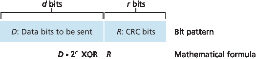
图 6.6 CRC
现在让我们讨论发送方如何计算 R。我们希望找到 R,使得存在一个 n 满足:
\(D⋅2^r \space \text{XOR} \space R = nG\)
即我们希望选择 R,使得 G 能整除 \(D⋅2^r \space \text{XOR} \space R\) 而无余数。如果我们对上述等式两边进行异或操作(即模2加法),我们得到:
\(D⋅2^r \space = \space nG \space \text{XOR} \space R\)
该等式表明,如果我们将 \(D⋅2^r\) 除以 G,所得余数正是 R。换句话说, R 可以计算为:
\(R = \text{remainder}\frac{D⋅2^r}{G}\)
图 6.7 展示了一个计算示例,其中 D=101110, d=6, G=1001, r=3。在该示例中发送的 9 位为 101110011。你可以自己验证这个计算,并检查是否确实有 \(D⋅2^r = 101011⋅G \space \text{XOR} \space R\)。
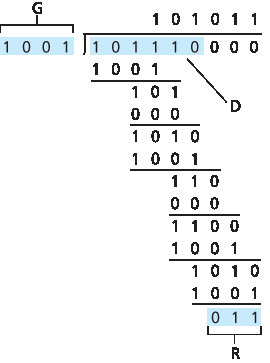
图 6.7 CRC 示例计算
目前已为 8 位、12 位、16 位和 32 位的生成多项式 G 定义了国际标准。 CRC-32 是一个 32 位标准,被多个链路层 IEEE 协议采纳,其生成多项式为:
GCRC-32 = 100000100110000010001110110110111
每个 CRC 标准都能检测长度小于 r+1 的突发错误。(即所有连续 r 位或更少位的错误都会被检测到)。此外,在合适的假设条件下,长度大于 r+1 的突发错误将以概率 \(1-0.5^r\) 被检测到。此外,每个 CRC 标准都能检测任意奇数个比特错误。关于 CRC 校验的实现讨论,详见 [Williams 1993]。CRC 码及更强大的编码方案背后的理论超出了本书的范围,参考文献 [Schwartz 1980] 为该主题提供了优秀的入门介绍。
An error-detection technique used widely in today’s computer networks is based on cyclic redundancy check (CRC) codes. CRC codes are also known as polynomial codes, since it is possible to view the bit string to be sent as a polynomial whose coefficients are the 0 and 1 values in the bit string, with operations on the bit string interpreted as polynomial arithmetic.
CRC codes operate as follows. Consider the d-bit piece of data, D, that the sending node wants to send to the receiving node. The sender and receiver must first agree on an r+1 bit pattern, known as a generator, which we will denote as G. We will require that the most significant (leftmost) bit of G be a 1. The key idea behind CRC codes is shown in Figure 6.6. For a given piece of data, D, the sender will choose r additional bits, R, and append them to D such that the resulting d+r bit pattern (interpreted as a binary number) is exactly divisible by G (i.e., has no remainder) using modulo-2 arithmetic. The process of error checking with CRCs is thus simple: The receiver divides the d+r received bits by G. If the remainder is nonzero, the receiver knows that an error has occurred; otherwise the data is accepted as being correct.
All CRC calculations are done in modulo-2 arithmetic without carries in addition or borrows in subtraction. This means that addition and subtraction are identical, and both are equivalent to the bitwise exclusive-or (XOR) of the operands. Thus, for example,
1011 XOR 0101 = 1110
1001 XOR 1101 = 0100
Also, we similarly have
1011 - 0101 = 1110
1001 - 1101 = 0100
Multiplication and division are the same as in base-2 arithmetic, except that any required addition or subtraction is done without carries or borrows. As in regular binary arithmetic, multiplication by \(2^k\) left shifts a bit pattern by k places. Thus, given D and R, the quantity D⋅2rXOR R yields the d+r bit pattern shown in Figure 6.6. We’ll use this algebraic characterization of the d+r bit pattern from Figure 6.6 in our discussion below.
Figure 6.6 CRC
Let us now turn to the crucial question of how the sender computes R. Recall that we want to find R such that there is an n such that
D⋅2rXOR R=nG
That is, we want to choose R such that G divides into D⋅2rXOR R without remainder. If we XOR (that is, add modulo-2, without carry) R to both sides of the above equation, we get
D⋅2r=nG XOR R
This equation tells us that if we divide D⋅2r by G, the value of the remainder is precisely R. In other words, we can calculate R as
R=remainderD⋅2rG
Figure 6.7 illustrates this calculation for the case of D=101110, d=6, G=1001, and r=3. The 9 bits transmitted in this case are 101 110 011. You should check these calculations for yourself and also check that indeed D⋅2r=101011⋅G XOR R.
Figure 6.7 A sample CRC calculation
International standards have been defined for 8-, 12-, 16-, and 32-bit generators, G. The CRC-32 32-bit standard, which has been adopted in a number of link-level IEEE protocols, uses a generator of
GCRC-32=100000100110000010001110110110111
Each of the CRC standards can detect burst errors of fewer than r+1 bits. (This means that all consecutive bit errors of r bits or fewer will be detected.) Furthermore, under appropriate assumptions, a burst of length greater than r+1 bits is detected with probability 1−0.5r. Also, each of the CRC standards can detect any odd number of bit errors. See [Williams 1993] for a discussion of implementing CRC checks. The theory behind CRC codes and even more powerful codes is beyond the scope of this text. The text [Schwartz 1980] provides an excellent introduction to this topic.